Python ‘Oceanic Nino Index’ HadSST4 tos anomalies#
Software requirements:
Python 3
python-cdo
numpy
matplotlib
cartopy
Example script#
ONI_Oceanic_Nino_Index_1950-2023.py
#!/usr/bin/env python
# coding: utf-8
'''
DKRZ example
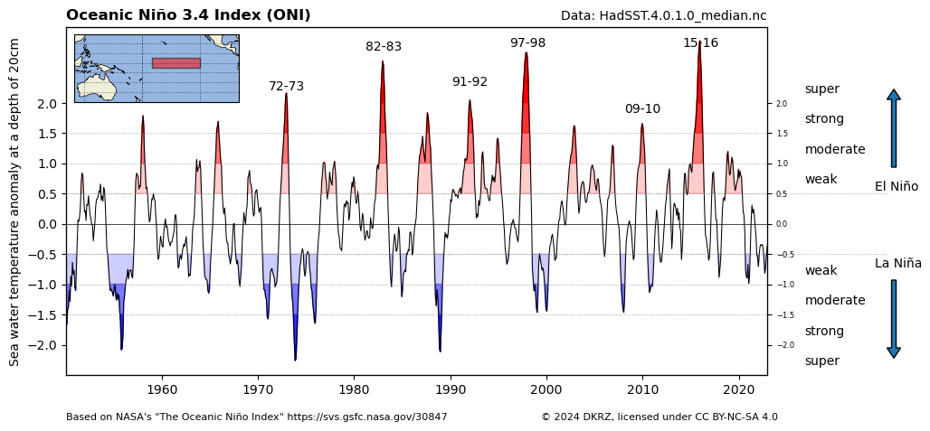
Plot Oceanic Nino Index (ONI)
This example script demonstrates how to draw the ONI time series data for the
Nino 3.4 area.
The resulting plot shows the time series of the ONI data from the HadSST.4.0.1
dataset available at https://www.metoffice.gov.uk/hadobs/hadsst4/data/download.html.
The plot was inspired by the animation 'The Oceanic Nino Index'
https://svs.gsfc.nasa.gov/30847 from NASA.
Description
Definition of the Oceanic Nino Index (ONI) from Climate Data Guide
(https://climatedataguide.ucar.edu/climate-data/nino-sst-indices-nino-12-3-34-4-oni-and-tni)
ONI (5N-5S, 170W-120W): The ONI uses the same region as the Niño 3.4 index.
The ONI uses a 3-month running mean, and to be classified as a full-fledged
El Niño or La Niña, the anomalies must exceed +0.5C or -0.5C for at least
five consecutive months. This is the operational definition used by NOAA.
Data
HadSST.4.0.1.0: From https://www.metoffice.gov.uk/hadobs/hadsst4/
"The Met Office Hadley Centre's sea surface temperature data set,
HadSST.4.0.1.0 is a monthly global field of SST on a 5° latitude by 5°
longitude grid from 1850 to date.
...
HadSST.4.0.1.0 is produced by taking in situ measurements of SST from ships
and buoys, rejecting measurements that fail quality checks, converting the
measurements to anomalies by subtracting climatological values from the
measurements, and calculating a robust average of the resulting anomalies on
a 5° by 5° degree monthly grid. After gridding the anomalies, bias adjustments
are applied to reduce the effects of changes in SST measuring practices."
-------------------------------------------------------------------------------
2024 copyright DKRZ licensed under CC BY-NC-SA 4.0
(https://creativecommons.org/licenses/by-nc-sa/4.0/deed.en)
-------------------------------------------------------------------------------
'''
import numpy as np
import matplotlib.pyplot as plt
from matplotlib.colors import ListedColormap
import matplotlib.patches as mpatches
import cartopy.crs as ccrs
import cartopy.feature as cfeature
from cdo import Cdo
cdo = Cdo()
# Function `fill_between_threshold()`
#
# Function to color data between value ranges.
def fill_between_threshold(ax, x, data, threshold, alpha):
if threshold >= 0.:
ax.fill_between(x.data,
data.where(data >= threshold).data,
threshold,
color='red',
alpha=alpha)
else:
ax.fill_between(x.data,
data.where(data <= threshold).data,
threshold,
color='blue',
alpha=alpha)
# Function `add_years_text_extremes()`
#
# Annotate the El Nino peaks with the year strings.
def add_years_text_extremes(ax, data, y=3.):
extremes = data[~np.isnan(data.where(data >= 1.5))]
year = 1800
for i in range(extremes.size):
if year != extremes.time.dt.year.data[i]:
y = extremes.data[i]
if extremes.time.dt.year.data[i] == year+1:
ystr = str(extremes.time.dt.year.data[i-1])[-2::] + \
'-' + str(extremes.time.dt.year.data[i])[-2::]
ax.text(extremes.time[i], y+0.2, ystr,ha='center',va='bottom')
year = extremes.time.dt.year.data[i]
else:
continue
# Function `main()`
def main():
# Extract Nino 3.4 area
#
# Extract the Nino 3.4 area from HadSST.4.0.1.0 data set and compute the field
# mean to get the time series data.
infile_sst = '../../data/HadSST.4.0.1.0_median.nc'
nino34_area = '190.,240.,-5.,5.'
ds_sst = cdo.fldmean(input='-sellonlatbox,'+nino34_area+' '+infile_sst,
options='--reduce_dim',
returnXDataset=True)
var = ds_sst.tos
time = ds_sst.time
# The computation of the 3-months running means leads to NaNs at time[0] and
# time[-1].
var = var.rolling(time=3, center=True).mean()
# Extract the time and data for the time range 1950-2023.
time_set = time.sel(time=slice('1950-01-01', '2023-01-01'))
var_set = var.sel(time=slice('1950-01-01', '2023-01-01'))
# Plotting
plt.switch_backend('agg')
fig, ax = plt.subplots(figsize=(10, 5))
ax.set_title('Oceanic Niño 3.4 Index (ONI)', loc='left', weight='bold')
ax.set_title('Data: HadSST.4.0.1.0_median.nc', loc='right', fontsize=10)
bottom, top = ax.set_ylim(-2.5, 3.25)
ax.set_xlim(time_set[0], time_set[-1])
ax.set_yticks(np.arange(-2.0, 2.5, 0.5))
ax.set_ylabel(var.long_name)
#-- threshold and alpha values
pthresh = np.arange(-2.0, 2.5, 0.5)
alpha = [0., 0.2, 0.4, 0.6, 0.9]
alpha = alpha[::-1] + alpha[1::]
#-- draw fill_between
for i in range(len(pthresh)):
fill_between_threshold(ax, time_set, var_set, pthresh[i], alpha[i])
#-- draw anomalies time series
ax.plot(time_set.data, var_set.data, color='black', lw=0.75)
#-- add year strings at the El Nino peaks
add_years_text_extremes(ax, var_set)
#-- add horizontal lines
for i in np.arange(-1.5, 2.0, 0.5):
if i == 0.:
ax.axhline( i, color='black', lw=0.5)
else:
ax.axhline( i, color='gray', lw=0.5, ls='dotted')
#-- add annotations on the right y-axis
ax2 = ax.twinx()
ax2.spines.right.set_position(('axes', 1.))
ax2.set_ylim(bottom, top)
ax2.set_yticks(ax.get_yticks())
ax2.yaxis.set_tick_params(labelsize=6)
#-- add gridlines
ax2.plot([ax.get_xticks().min(), ax.get_xticks().max()+2000],[0.5, 0.5],
color='gray', lw=0.5, ls='dotted', clip_on=False, zorder=-10)
ax2.plot([ax.get_xticks().min(), ax.get_xticks().max()+2000],[-0.5, -0.5],
color='gray', lw=0.5, ls='dotted', clip_on=False, zorder=-10)
#-- add text
ax2.text(ax.get_xticks().max()+1500, 0.5, 'El Niño', va='bottom')
ax2.text(ax.get_xticks().max()+1500, -0.55, 'La Niña', va='top')
#-- add arrows on the right side
arrow_up = mpatches.FancyArrow(1.04, 0.57, 0., 0.15, width=0.005,
figure=fig, clip_on=False,
transform=fig.transFigure)
arrow_down = mpatches.FancyArrow(1.04, 0.32, 0., -0.15, width=0.005,
figure=fig, clip_on=False,
transform=fig.transFigure)
ax2.add_patch(arrow_up)
ax2.add_patch(arrow_down)
#-- add right axis ticks, labels, and text
ax3 = ax.twinx()
ax3.set_ylim(bottom,top)
ax3.set_yticks([-2.25, -1.75, -1.25, -0.75,
0.75, 1.25, 1.75, 2.25])
ax3.set_yticklabels(['super', 'strong', 'moderate', 'weak',
'weak', 'moderate', 'strong', 'super'])
ax3.tick_params(axis='both', which='both', length=0, pad=30)
#-- add copyright and other informations
plt.text(0.65, 0.01, '© 2024 DKRZ, licensed under CC BY-NC-SA 4.0',
fontsize=8, transform=plt.gcf().transFigure)
plt.text(0.125, 0.01,
'Based on NASA\'s "The Oceanic Niño Index" https://svs.gsfc.nasa.gov/30847 ',
fontsize=8, ha='left', transform=plt.gcf().transFigure)
#-- add small map to upper left of the axis
pos_map = [ax.get_position().x0-0.05, ax.get_position().y1 - 0.165, 0.3, 0.15]
ax4 = fig.add_axes(pos_map, autoscalex_on=False,
projection=ccrs.PlateCarree(central_longitude=180)) #-- x,y,w,h
ax4.set_extent([-250, -80, -40, 30], crs=ccrs.PlateCarree())
ax4.coastlines(linewidth=0.5)
ax4.add_feature(cfeature.LAND)
ax4.add_feature(cfeature.OCEAN)
ax4.add_patch(mpatches.Rectangle(xy=[190, -5], width=50, height=10,
fc='red', ec='k', alpha=0.5,
transform=ccrs.PlateCarree()))
gl = ax4.gridlines(draw_labels=False, lw=0.5, alpha=0.4, color='k', ls='--')
#-- save figure
plt.savefig('plot_oceanic_nino_index_ONI_time_series_1950-2023.png',
bbox_inches='tight', facecolor='white')
# Delete temporary files
#
# **Note**: It is always a good idea to delete the temporary files, as they
# are not always deleted automatically when the script is finished.
cdo.cleanTempDir()
if __name__ == '__main__':
main()
Plot result#