Python animation with ffmpeg#
Software requirements:
Python 3
numpy
xarray
matplotlib
cartopy
ffmpeg
Example script#
animation_with_ffmpeg_normal_and_faster.py
#!/usr/bin/env python
# coding: utf-8
'''
DKRZ tutorial

Animation of geospatial data

It is quite easy to create a video with Matplotlib and FFmpeg from time-
dependent data. In this notebook the deployment of the temperature data over
time is shown using two slightly different ways, which differ significantly
in runtime.

Note:
  In case of problems with FFmpeg it is advisable to install the latest
  version and set the ffmpeg_path via plt.rcParams to animation.ffmpeg_path
  as already used in this notebook.

Content

- Create the animation as usual  (run time: 16.4s)
- Create the animation 8x faster (run time:  1.9s)
- save the animation in mpeg4 file

The example input file _rectilinear_grid_2D.nc_ can be downloaded from
      https://nextcloud.dkrz.de/s/WHGZgCWrZLPnpBn

FFmpeg home page: https://ffmpeg.org/

-------------------------------------------------------------------------------
2022 copyright DKRZ licensed under CC BY-NC-SA 4.0
               (https://creativecommons.org/licenses/by-nc-sa/4.0/deed.en)
-------------------------------------------------------------------------------
'''
import time, os
import numpy as np
import xarray as xr

import matplotlib.pyplot as plt
from matplotlib.animation import FuncAnimation
from matplotlib import animation
import cartopy.crs as ccrs

def main():
    # Set the path of the ffmpeg binary, e.g. in a 'cartopy' conda environment
    ffmpeg_path = os.environ['HOME']+'/miniconda3/envs/cartopy/bin/ffmpeg'
    plt.rcParams['animation.ffmpeg_path'] = ffmpeg_path

    # Open data set
    infile = '../../data/rectilinear_grid_2D.nc'
    ds = xr.open_dataset(infile)

    # Read the data and coordinate variables.
    lon = ds.lon
    lat = ds.lat
    var = ds.tsurf

    # Set plotting parameters
    # -----------------------
    # Use the dictionary `plot_parameter` to define some plot settings.
    plot_parameter = {}
    plot_parameter['extent'] = [-180, 180, -90, 90]
    plot_parameter['projection'] = ccrs.PlateCarree()
    plot_parameter['vmin'] = 240.
    plot_parameter['vmax'] = 300.
    plot_parameter['cmap'] = 'RdBu_r'
    plot_parameter['title'] = var.long_name

    # Get number of frames
    # --------------------
    # The input dataset contains 40 time steps and we want to create the animation
    # over all.
    frames = ds.time.size

    # Get date strings
    # ----------------
    # The date string should be added on top of the plot and therefore we get the
    # date strings in a nicer notation.
    time_str = ds.time.dt.strftime('%Y-%m-%d').data

    #------------------------------------------------------------------------------
    # Define function plot_init()
    #
    # This function is needed as input for the `init_func` parameter of
    # Matplotlib's `FuncAnimation`. It presets in this case the extent of the
    # map, the title  and coastline drawing.
    #------------------------------------------------------------------------------
    def plot_init():
        ax.set_extent(plot_parameter['extent'])
        ax.coastlines()
        plt.title(plot_parameter['title'], fontsize=20)
        return plot

    #------------------------------------------------------------------------------
    # Create the animation as usual
    # -----------------------------
    # We use Matplotlib's `FuncAnimation` routine to make an animation from the
    # time-dependent variable _surface temperature_. `FuncAnimation` needs as
    # second input parameter a _function to call at each frame_. In this case we
    # define the function `update_frame()` for creating a plot for a given
    # timestep (frame).

    #------------------------------------------------------------------------------
    # Define function update_frame()
    #
    # This is the function that is called for each time step (frame) to generate
    # the corresponding plot.
    #------------------------------------------------------------------------------
    def update_frame(frame):
        plot = ax.pcolormesh(lon, lat, var[frame,:,:],
                         cmap=plot_parameter['cmap'],
                         vmin=plot_parameter['vmin'],
                         vmax=plot_parameter['vmax'])
        tx.set_text(time_str[frame])
        return plot, tx

    # Create the animation I
    # ----------------------
    # Now, we can generate the animation doing the following steps:
    #
    # 1. define figure and axis
    # 2. create the plot object for the first time step
    # 3. add a colorbar
    # 4. add the date string on top
    # 5. create the animation in memory
    # 6. save the animation to a mpeg4 file
    t1 = time.time()

    fig, ax = plt.subplots(figsize=(16,6),
                           subplot_kw={"projection": plot_parameter['projection']})

    plot = ax.pcolormesh(lon, lat, var[0,:,:],
                         cmap=plot_parameter['cmap'],
                         vmin=plot_parameter['vmin'],
                         vmax=plot_parameter['vmax'])
    cb = plt.colorbar(plot)
    tx = fig.text(0.69, 0.89, time_str[0])

    ani = FuncAnimation(fig, update_frame, frames=range(0, frames),
                         init_func=plot_init)

    ani.save('tsurf_animation.mp4',
             writer=animation.FFMpegWriter(fps=60, bitrate=5000, codec='h264'),
             dpi=100)

    t2 = time.time()
    print('run time: '+str(t2-t1))

    #------------------------------------------------------------------------------
    # Create the animation 8x faster
    # ------------------------------
    # Instead of creating a new plot for each time step, we only exchange the
    # data array for the plot in the `update_frame2()` function with Matplotlib's
    # `plot.set_array()` method. This makes the creation of the animation much
    # faster.

    #------------------------------------------------------------------------------
    # Define function update_frame2()
    #
    # Exchange the data array of the plot with Matplotlib's `plot.set_array()`
    # method. This makes the creation of the animation much faster.
    #------------------------------------------------------------------------------
    def update_frame2(frame):
        plot.set_array(np.array(var[frame,:,:]).ravel())
        tx.set_text(time_str[frame])
        return plot, tx

    # Create the animation II
    # -----------------------
    # Same as above but this time we use the `update_frame2()` function to create
    # the animation with Matplotlib's `FuncAnimation`.
    #
    # 1. define figure and axis
    # 2. create the plot object for the first time step
    # 3. add a colorbar
    # 4. add the date string on top
    # 5. create the animation in memory
    # 6. save the animation to a mpeg4 file
    t1 = time.time()

    fig, ax = plt.subplots(figsize=(16,6),
                           subplot_kw={"projection": plot_parameter['projection']})

    plot = ax.pcolormesh(lon, lat, var[0,:,:],
                         cmap=plot_parameter['cmap'],
                         vmin=plot_parameter['vmin'],
                         vmax=plot_parameter['vmax'])
    cb = plt.colorbar(plot)
    tx = fig.text(0.69, 0.89, time_str[0])

    ani = FuncAnimation(fig, update_frame2, frames=range(0, frames),
                         init_func=plot_init)

    ani.save('tsurf_animation.mp4',
             writer=animation.FFMpegWriter(fps=60, bitrate=5000, codec='h264'),
             dpi=100)

    t2 = time.time()
    print('run time: '+str(t2-t1))


if __name__ == '__main__':
    main()
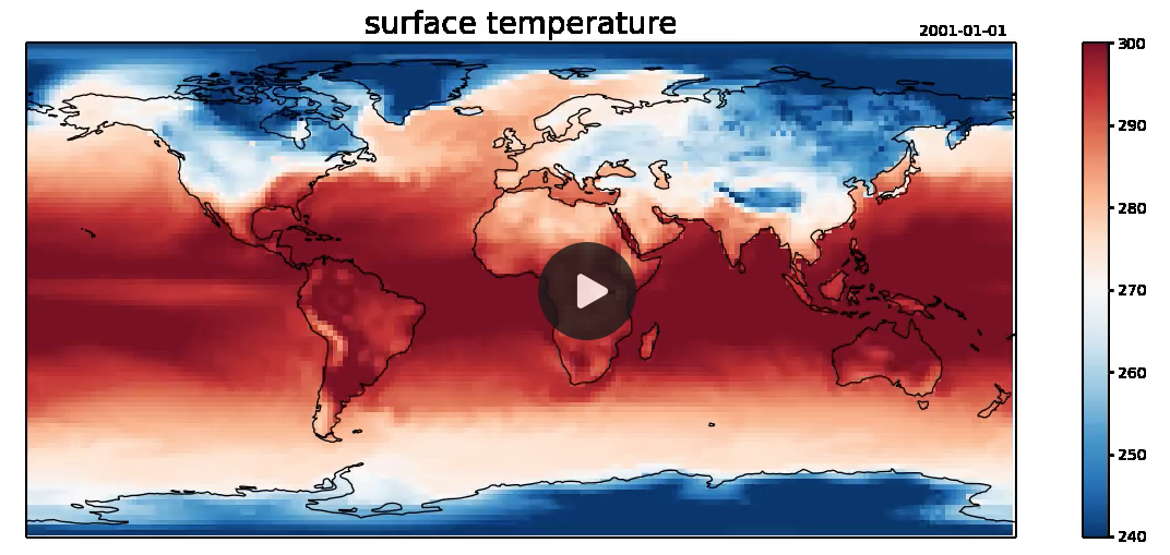
Plot result#