Python: Data clipping with a shapefile#
Description
This example shows how to use the geometries of a shapefile to clip data outside these geometries (polygons), in this case one or more states. Actually, it is not clipping, but rather covering the unwanted outer regions. This allows us to have a clean representation at the boundary lines.
Content
Receive the NaturalEarth shapefile
Clip data for single country - Receive the topography dataset - Extract polygons - Create colormap - Plotting
Clip data for multiple countries - Receive totpography data - Extract polygons - Plotting
Software requirements
Python 3
numpy
matplotlib
cartopy
geopandas
shapely
python-cdo
Example script#
data_clipping_with_shapefile_1.py
#!/usr/bin/env python
# coding: utf-8
#
# Data clipping with a shapefile
#
#------------------------------------------------------------------------------
# 2025 copyright DKRZ licensed under CC BY-NC-SA 4.0
#------------------------------------------------------------------------------
#
# This example shows how to use the geometries of a shapefile to clip data
# outside these geometries (polygons), in this case one or more states. Actually,
# it is not clipping, but rather covering the unwanted outer regions. This
# allows us to have a clean representation at the boundary lines.
#
# We want to create the topography map of one or more selected states. To receive
# the topography dataset we use CDO (https://code.mpimet.mpg.de/projects/cdo)
# with the operator `topo` and extract only the data for the chosen region of
# the wanted states with the operator `sellonlatbox`.
#
# The shapefile containing the geometries of the state borders can be received
# using Cartopy's `cartopy.io.shapereader` function that does the download from
# `Natural Earth` under the hood when it is not already done.
#
# Content
# - Receive the NaturalEarth shapefile
# - Clip data for single country
# - Receive the topography dataset
# - Extract polygons
# - Create colormap
# - Plotting
# - Clip data for multiple countries
# - Receive totpography data
# - Extract polygons
# - Plotting
#------------------------------------------------------------------------------
import numpy as np
from shapely.geometry import Polygon
import geopandas
import matplotlib.pyplot as plt
import matplotlib.colorbar as colorbar
import matplotlib.colors as mcolors
import cartopy.crs as ccrs
import cartopy.feature as cfeature
from cartopy.io import shapereader
from cdo import Cdo
cdo = Cdo()
#------------------------------------------------------------------------------
#-- Receive the NaturalEarth shapefile
#--
#-- We use Cartopy to get the cultural/admin shapefile that contains the country
#-- border lines of each country in the world. The shapefile then will be read
#-- using `geopandas.read_file`.
#--
#-- Ther border geometries are stored in the cultural admin_0_countries shapefiles
#-- with different resolutions, here we need the high resolution '10m' data.
#------------------------------------------------------------------------------
resolution = '10m'
category = 'cultural'
name = 'admin_0_countries'
shapefile_name = shapereader.natural_earth(resolution, category, name)
df = geopandas.read_file(shapefile_name)
#-- get country names of the column 'ADMIN'
all_countries = np.sort([ s for s in df['ADMIN'] ])
print(shapefile_name)
#print(all_countries)
#-- Clip data for single country
#--
#-- Receive the topography dataset
#--
#-- The `CDO` operator `topo` is used to retrieve the topography on a global
#-- 0.1°x0.1° grid and extract the wanted region. This makes the computation of
#-- the polygons much faster.
#-- set extent
lonmin, lonmax = 5., 16.
latmin, latmax = 47., 55.5
ds = cdo.sellonlatbox(f'{lonmin},{lonmax},{latmin},{latmax}',
input='-topo,global_0.1',
returnXDataset=True)
topo = ds.topo
print(topo)
#-- Extract polygons
#--
#-- Now, we can search and extract the polygons representing the German
# borderline. If you want to extract the geometries for multiple countries see
# at 'Clip data for multiple countries` below.
country_list = ['Germany']
poly = [df.loc[df['ADMIN'] == country_list[0]]['geometry'].values[0]]
#-- Create colormap
#--
#-- Create a new colormap for the topography data.
colors_greens = plt.cm.YlGn(np.linspace(0.2, 0.9, 5))
colors_browns = plt.cm.copper_r(np.linspace(0.3, 0.9, 5))
colors_white = plt.cm.Greys_r(np.linspace(0.95, 1., 1))
all_colors = np.vstack((colors_greens, colors_browns, colors_white))
cmap = mcolors.LinearSegmentedColormap.from_list('topo_map', all_colors)
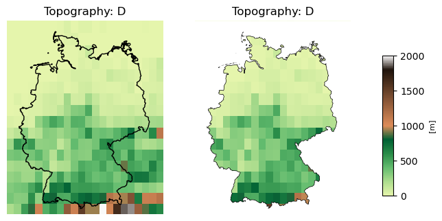
#-- Plotting
#--
#-- The left plot shows the topography data with the shapefile geometries
# overlayed on the map. The middle plot adds a mask that covers the data outside
# Germany's borders, and the right plot shows a common colorbar.
#-- projections
proj = ccrs.Mercator()
crs = ccrs.PlateCarree()
#-- data range for colors
vmin, vmax = 0, 2000
norm = mcolors.Normalize(vmin=vmin, vmax=vmax)
#-- title
title = 'Topography: D'
#-- create the plots
fig, (ax1,ax2,ax3) = plt.subplots(nrows=1, ncols=3, figsize=(10,8),
subplot_kw=dict(projection=ccrs.Mercator()))
#----------------------
#---- ax1 ----
#----------------------
ax1.set_title(title)
ax1.axis('off')
ax1.add_geometries(poly, crs=crs, facecolor='none', edgecolor='black')
ax1.set_extent([lonmin, lonmax, latmin, latmax], crs=crs)
#-- plot topography data
plot1 = ax1.pcolormesh(ds.lon, ds.lat, topo,
norm=norm,
cmap=cmap,
transform=crs)
#----------------------
#---- ax2 ----
#----------------------
ax2.set_title(title)
ax2.axis('off')
ax2.add_geometries(poly, crs=crs, facecolor='none', edgecolor='black')
ax2.set_extent([lonmin, lonmax, latmin, latmax], crs=crs)
#-- base polygon is a rectangle, another polygon is simplified Germany
def generate_rectangle_bounds(x0, x1, y0, y1):
xnew = [x1,x0,x0,x1,x1]
ynew = [y1,y1,y0,y0,y1]
rect = [(x,y) for x,y in zip(xnew,ynew)]
return rect
tolerance = 0
mask = Polygon(generate_rectangle_bounds(lonmin, lonmax, latmin, latmax)).difference(poly[0].simplify(tolerance))
mask_proj = proj.project_geometry(mask, crs)
#-- plot topography data
plot2 = ax2.pcolormesh(ds.lon, ds.lat, topo,
norm=norm,
cmap=cmap,
transform=crs)
#-- add the mask with alpha=1
ax2.add_geometries(mask_proj, proj, zorder=12, facecolor='white', edgecolor='none',
alpha=1)
#---- ax3 ----
#-- create the common colorbar in the second last axis
ax3.set_visible(False)
bbox = ax3.get_position()
x,y,w,h = bbox.x0, bbox.y0, bbox.width, bbox.height
cax = fig.add_axes([x, y, w/14, h-0.03], autoscalex_on=True)
cbar = colorbar.Colorbar(cax, orientation='vertical', cmap=cmap, norm=norm, alpha=1)
cbar.set_label(label='[m]', size=8)
#-- save plot
plt.savefig('plot_data_clipping_with_shapefile.png', bbox_inches='tight',
facecolor='white')
plt.show()
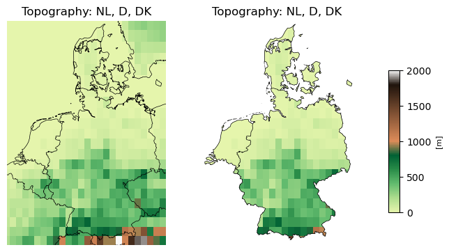
#-- Clip data for multiple countries
#--
#-- In the next example we create the topography plots for 3 different countries,
#-- here Netherlands, Germany, and Denmark.
#-- Receive the topography data
#-- extent
lonmin, lonmax = 2.8, 15.5
latmin, latmax = 47., 57.9
ds = cdo.sellonlatbox(f'{lonmin},{lonmax},{latmin},{latmax}',
input='-topo,global_0.1',
returnXDataset=True)
topo = ds.topo
print(topo)
#-- Extract polygons
country_list = ['Denmark', 'Germany', 'Netherlands']
#-- get the polygons
if len(country_list) > 1:
tmp = df[ df['ADMIN'].isin(country_list) ].dissolve(by='LEVEL')
poly = [tmp['geometry'].values[0]]
else:
poly = [df.loc[df['ADMIN'] == country_list[0]]['geometry'].values[0]]
#-- Plotting
#-- projections
proj = ccrs.Mercator()
crs = ccrs.PlateCarree()
#-- data range for colors
vmin, vmax = 0, 2000
norm = mcolors.Normalize(vmin=vmin, vmax=vmax)
#-- title
title = 'Topography: NL, D, DK'
#-- create the plot
fig, (ax1,ax2,ax3) = plt.subplots(nrows=1, ncols=3, figsize=(10,8),
subplot_kw=dict(projection=ccrs.Mercator()))
#----------------------
#---- ax1 ----
#----------------------
ax1.set_title(title)
ax1.axis('off')
ax1.set_extent([lonmin, lonmax, latmin, latmax])
#-- plot topography data
plot1 = ax1.pcolormesh(ds.lon, ds.lat, topo,
norm=norm,
cmap=cmap,
transform=crs)
#-- outline of the extracted polygon
#ax1.add_geometries(poly, crs=crs, facecolor='none', edgecolor='black')
ax1.add_feature(cfeature.BORDERS.with_scale('10m'), ls='-', ec='k', lw=0.5)
ax1.add_feature(cfeature.COASTLINE.with_scale('10m'), ls='-', ec='k', lw=0.5)
#----------------------
#---- ax2 ----
#----------------------
ax2.set_title(title)
ax2.axis('off')
ax2.add_geometries(poly, crs=crs, facecolor='none', edgecolor='black')
ax2.set_extent([lonmin, lonmax, latmin, latmax])
#-- base polygon is a rectangle, another polygon is simplified Germany
def generate_rectangle_bounds(x0, x1, y0, y1):
xnew = [x1,x0,x0,x1,x1]
ynew = [y1,y1,y0,y0,y1]
rect = [(x,y) for x,y in zip(xnew,ynew)]
return rect
tolerance = 0
mask = Polygon(generate_rectangle_bounds(lonmin, lonmax, latmin, latmax)).difference(poly[0].simplify(tolerance))
mask_proj = proj.project_geometry(mask, crs)
#-- plot topography data
plot2 = ax2.pcolormesh(ds.lon, ds.lat, topo,
norm=norm,
cmap=cmap,
transform=crs)
#-- add borderlines
ax2.add_feature(cfeature.BORDERS.with_scale('10m'), ls='-', ec='k', lw=0.5)
#-- add the mask with alpha=1
ax2.add_geometries(mask_proj, proj, zorder=12, facecolor='white', edgecolor='none',
alpha=1)
#---- ax3 ----
#-- create the common colorbar in the second last axis
ax3.set_visible(False)
bbox = ax3.get_position()
x,y,w,h = bbox.x0, bbox.y0, bbox.width, bbox.height
cax = fig.add_axes([x, y, w/14, h-0.03], autoscalex_on=True)
cbar = colorbar.Colorbar(cax, orientation='vertical', cmap=cmap, norm=norm,
alpha=1)
cbar.set_label(label='[m]', size=8)
#-- save plot
plt.savefig('plot_data_clipping_with_shapefile_2.png', bbox_inches='tight',
facecolor='white')
plt.show()
Plot result#