Python different anomalies#
Software requirements:
Python 3
Xarray
SciPy
Pandas
Matplotlib
Example script#
anomalies_North_Germany.py
#!/usr/bin/env python
# coding: utf-8
'''
DKRZ example
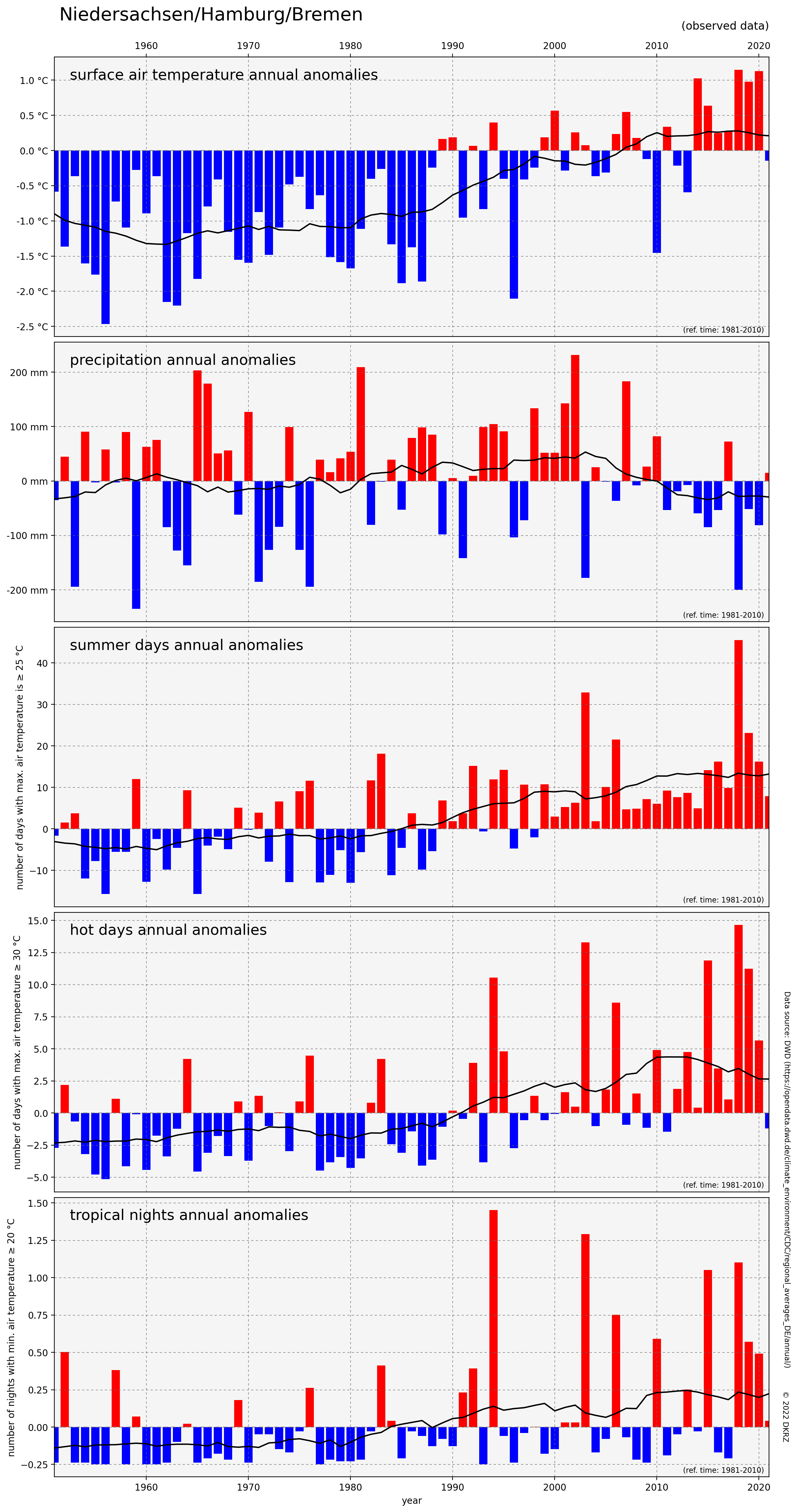
Draw the anomalies of air temperatur, precipitation, summer days, hot days,
and tropical nights.
Data source:
https://opendata.dwd.de/climate_environment/CDC/regional_averages_DE/annual/
DWD weather dictionary:
https://www.dwd.de/DE/service/lexikon/lexikon_node.html
Variables frequency time range
----------------------------------------------------
air temperature mean annual 1881 - 2021
precipitation annual 1881 - 2021
tropical nights annual 1951 - 2021
summer days annual 1951 - 2021
hot_days annual 1951 - 2021
-------------------------------------------------------------------------------
2021 copyright DKRZ licensed under CC BY-NC-SA 4.0 <br>
(https://creativecommons.org/licenses/by-nc-sa/4.0/deed.en)
-------------------------------------------------------------------------------
'''
import numpy as np
import pandas as pd
import scipy.signal
import matplotlib.pyplot as plt
import matplotlib.gridspec as gridspec
from matplotlib.ticker import StrMethodFormatter
#---------------------------------------------------------------------------
# Function to calculate the anomalies
#---------------------------------------------------------------------------
def calc_anomalies(data, reftime, name='Deutschland'):
ref_i = data.index[data.Jahr == reftime[0]]
ref_j = data.index[data.Jahr == reftime[1]]
ref_data = data.loc[range(ref_i.values[0],ref_j.values[0]+1)][name]
climatology = ref_data.mean()
anomaly = data.Deutschland - climatology
return anomaly
#---------------------------------------------------------------------------
# Function to calculate the running mean
# The Savitzky-Golay filter uses convolution process applied on an array for
# smoothing. The Python package scipy provide the function as shown in the
# next example.
#---------------------------------------------------------------------------
def calc_running_mean(data, window_length=30, polyorder=3, mode='nearest'):
return scipy.signal.savgol_filter(data,
window_length,
polyorder,
mode='nearest')
#---------------------------------------------------------------------------
# Function to create one plot of the gridspec panel
#---------------------------------------------------------------------------
def create_plot(ax, x, data, uppertitle='', lowertitle='', xlabel='', ylabel='',
refline=False, plotstyle='line'):
ax.set_facecolor('whitesmoke')
colors = ['red' if (value > 0) else 'blue' for value in data]
if plotstyle == 'bar':
ax.bar(x, data, color=colors)
else:
ax.plot(x, data, linestyle='-', color='blue', linewidth=1)
if refline:
plt.axhline(y=0., color='gray', linestyle=(0, (5, 5)), linewidth=0.8)
ax.plot(x, calc_running_mean(data), color='black', linewidth=1.5)
ax.grid(linestyle=(0, (5, 5)), linewidth=0.5, color='dimgray')
ax.set_xlim(x.values[0], x.values[-1])
ax.set_xlabel(xlabel)
ax.set_ylabel(ylabel)
xmin, xmax = ax.get_xlim()
ymin, ymax = ax.get_ylim()
ax.text(xmin+1.5, ymax-(ymax-ymin)*0.04, uppertitle, fontsize=16,
ha='left', va='top')
ax.text(xmax-0.5, ymin+(ymax-ymin)*0.01, lowertitle, fontsize=8,
ha='right', va='bottom')
#----------
# Main
#----------
def main():
#-- Which state do we want to plot?
states = 'Niedersachsen/Hamburg/Bremen'
#-- To get a better comparison of the anomalies we extract the same time range
#-- for temperature and precipitation
sel_time = [1951,2021]
#-- Reference time range for the 30 years climatology
ref_time = [1981,2010]
#---------------------------------------------------------------------------
# Air temperature (annual mean) in °C (2 m altitude).
# Read the CSV data from DWD with Pandas.
#---------------------------------------------------------------------------
temp_file = '../../data/regional_averages_tm_year.txt'
temp = pd.read_csv(temp_file, header=1, sep=';')
#-- Get the indices for the selected time range that applies to all variables
t_i = temp.index[temp.Jahr == sel_time[0]]
t_j = temp.index[temp.Jahr == sel_time[1]]
# Extract the temperature data for the selected time range
temp_sel = temp.loc[range(t_i[0],t_j[0]+1)]
#-- Compute the temperature anomalies
anomaly_temp_sel = calc_anomalies(temp_sel, reftime=ref_time, name=states)
#---------------------------------------------------------------------------
# Precipitation (annual mean) in mm.
#---------------------------------------------------------------------------
prec_file = '../../data/regional_averages_rr_year.txt'
prec = pd.read_csv(prec_file, header=1, sep=';')
#-- Extract the precipitation data for the selected time range
prec_sel = prec.loc[range(t_i.values[0],t_j.values[0]+1)]
#-- Compute the precipitation anomalies
anomaly_prec_sel = calc_anomalies(prec_sel, reftime=ref_time, name=states)
#---------------------------------------------------------------------------
# Summer days (annual mean)
#
# DWD: 'A summer day is a day when the maximum air temperature is ≥ 25 °C.
# The number of summer days also includes the subset of hot days. The number
# of summer days supplements the statements on the quality of a summer, which
# is primarily determined on the basis of the number of hot days.'
#---------------------------------------------------------------------------
summer_file = '../../data/regional_averages_txas_year.txt'
summer = pd.read_csv(summer_file, header=1, sep=';')
#-- Compute the tropical nights anomalies
anomaly_summer = calc_anomalies(summer, reftime=ref_time, name=states)
#---------------------------------------------------------------------------
# Hot Days (annual mean)
#
# DWD: 'A Hot Day is a day on which the maximum air temperature is ≥ 30 °C.
# A hot day was also called a tropical day in the past.'
#---------------------------------------------------------------------------
hotd_file = '../../data/regional_averages_txbs_year.txt'
hotd = pd.read_csv(hotd_file, header=1, sep=';')
#-- Compute the hot days anomalies
anomaly_hotd = calc_anomalies(hotd, reftime=ref_time, name=states)
#---------------------------------------------------------------------------
# Tropical nights (annual mean)
#
# DWD: 'A tropical night is a night in which the minimum air temperature
# is ≥ 20 °C (daily measurement period: 18 UTC to 06 UTC ). At most
# DWD stations, there is an average of less than one tropical night
# per year. At individual very favorably located stations, 2 to 3
# annual tropical nights are registered.'
#---------------------------------------------------------------------------
tropic_file = '../../data/regional_averages_tnes_year.txt'
tropic = pd.read_csv(tropic_file, header=1, sep=';')
#-- Compute the tropical nights anomalies
anomaly_tropic = calc_anomalies(tropic, reftime=ref_time, name=states)
#---------------------------------------------------------------------------
#-- Plot all anomalies on one page
#-- Draw all anomalies plots under each other and save the figure in a PNG file.
#---------------------------------------------------------------------------
plt.switch_backend('agg')
fig = plt.figure(figsize=(14,28))
gs = gridspec.GridSpec(5, 1, figure=fig, height_ratios = [1,1,1,1,1], hspace=0.02)
plt.rcParams['xtick.top'] = plt.rcParams['xtick.labeltop'] = True
plt.rcParams['xtick.bottom'] = plt.rcParams['xtick.labelbottom'] = False
#-- temperature anomalies
ax0 = fig.add_subplot(gs[0,:])
create_plot(ax0, temp_sel.Jahr, anomaly_temp_sel,
uppertitle='surface air temperature annual anomalies',
lowertitle='(ref. time: '+str(ref_time[0])+'-'+str(ref_time[1])+')',
xlabel='year',
refline=True,
plotstyle='bar')
ax0.set_xlabel('')
ax0.yaxis.set_major_formatter(StrMethodFormatter(u"{x:.1f} °C"))
plt.rcParams['xtick.top'] = plt.rcParams['xtick.labeltop'] = False
plt.rcParams['xtick.bottom'] = plt.rcParams['xtick.labelbottom'] = False
#-- precipitation anomalies
ax1 = fig.add_subplot(gs[1,:])
create_plot(ax1, prec_sel.Jahr, anomaly_prec_sel,
uppertitle='precipitation annual anomalies',
lowertitle='(ref. time: '+str(ref_time[0])+'-'+str(ref_time[1])+')',
xlabel='year',
refline=True,
plotstyle='bar')
ax1.set_xlabel('')
ax1.yaxis.set_major_formatter(StrMethodFormatter(u"{x:.0f} mm"))
#-- summer days anomalies
ax2 = fig.add_subplot(gs[2,:])
create_plot(ax2, summer.Jahr, anomaly_summer,
uppertitle='summer days annual anomalies',
lowertitle='(ref. time: '+str(ref_time[0])+'-'+str(ref_time[1])+')',
xlabel='year',
ylabel='number of days with max. air temperature is ≥ 25 °C',
refline=True,
plotstyle='bar')
ax2.set_xlabel('')
#-- hot days anomalies
ax3 = fig.add_subplot(gs[3,:])
create_plot(ax3, hotd.Jahr, anomaly_hotd,
uppertitle='hot days annual anomalies',
lowertitle='(ref. time: '+str(ref_time[0])+'-'+str(ref_time[1])+')',
xlabel='year',
ylabel='number of days with max. air temperature ≥ 30 °C',
refline=True,
plotstyle='bar')
ax3.set_xlabel('')
plt.rcParams['xtick.bottom'] = plt.rcParams['xtick.labelbottom'] = True
#-- tropical nights anomalies
ax4 = fig.add_subplot(gs[4,:])
create_plot(ax4, tropic.Jahr, anomaly_tropic,
uppertitle='tropical nights annual anomalies',
lowertitle='(ref. time: '+str(ref_time[0])+'-'+str(ref_time[1])+')',
xlabel='year',
ylabel='number of nights with min. air temperature ≥ 20 °C',
refline=True,
plotstyle='bar')
#-- ad some text
plt.figtext(0.13, 0.9, states, ha='left', fontsize=20)
plt.figtext(0.9, 0.895, '(observed data)', ha='right', fontsize=12)
plt.figtext(0.913, 0.13, '© 2022 DKRZ',
rotation=270, fontsize=8)
plt.figtext(0.915, 0.17,
'Data source: DWD (https://opendata.dwd.de/climate_environment/CDC/regional_averages_DE/annual/)',
rotation=270, fontsize=8)
#-- write plot to PNG file
plt.savefig('plot_different_anomalies_North_Germany.png', bbox_inches='tight',
facecolor='white')
if __name__ == '__main__':
main()
Plot result: