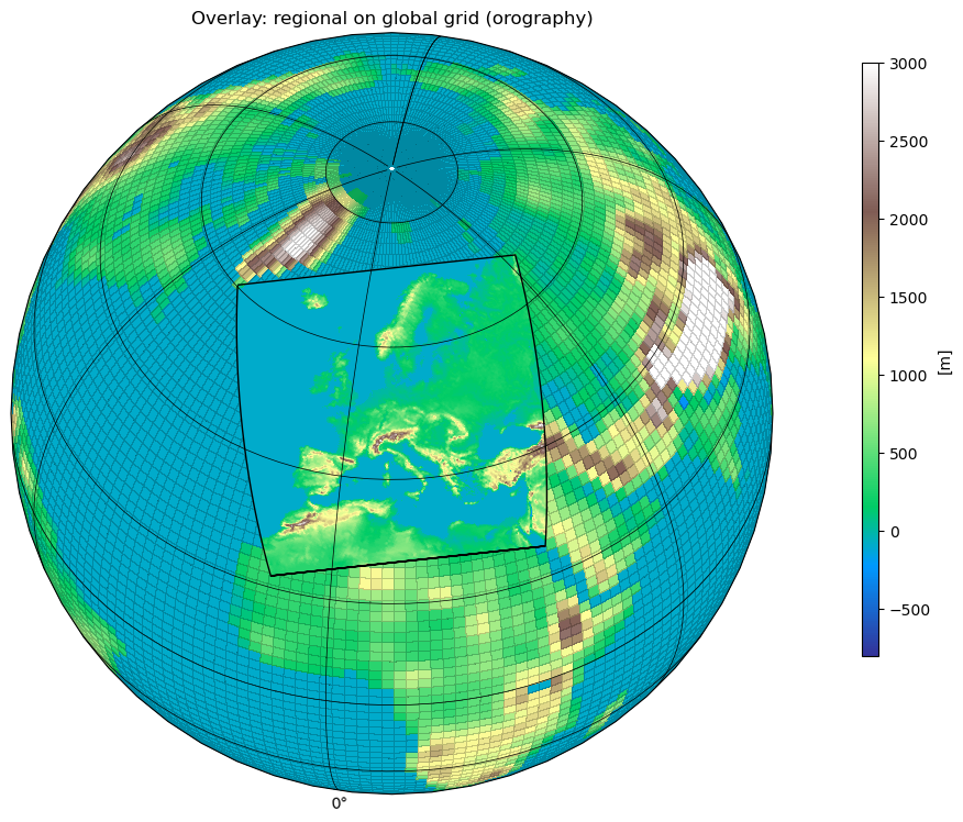
Python overlay regional on global grid#

Software requirements:

Python 3
Numpy
matplotlib
cartopy
xarray

Projection: - Orthographic

Grids:

The first grid is a coarse global grid (CMIP5)
- grid type: lonlat
- points=18432 (192x96)
- lon : 0 to 358.125 by 1.875 degrees_east circular
- lat : -88.57217 to 88.57217 degrees_north
The second grid is a high resolution regional grid (CORDEX EUR-11)
- grid type: curvilinear
- points=174688 (424x412)
- lon : -44.59386 to 64.96438 degrees_east
- lat : 21.98783 to 72.585 degrees_north

Example script#

overlay_regional_on_global_grid.py

#!/usr/bin/env python
# coding: utf-8
'''
DKRZ example

Draw two grids with different resolutions

Used packages:
    - numpy
    - xarray
    - matplotlib
    - cartopy

Projection:
    - Orthographic

Grids:
1. The first grid is a coarse global grid (CMIP5)

    grid type: lonlat
    points=18432 (192x96)
    lon : 0 to 358.125 by 1.875 degrees_east  circular
    lat : -88.57217 to 88.57217 degrees_north

2. The second grid is a high resolution regional grid (CORDEX EUR-11)

    grid type: curvilinear
    points=174688 (424x412)
    lon : -44.59386 to 64.96438 degrees_east
    lat : 21.98783 to 72.585 degrees_north

-------------------------------------------------------------------------------
2021 copyright DKRZ licensed under CC BY-NC-SA 4.0 <br>
               (https://creativecommons.org/licenses/by-nc-sa/4.0/deed.en)
-------------------------------------------------------------------------------
'''
import numpy as np
import xarray as xr
import cartopy.crs as ccrs
import cartopy.feature as cfeature
import cartopy.util as cutil
import matplotlib.pyplot as plt
import matplotlib.patches as mpatches

def main():
    #-- Read global data:
    orog_file1 = "../../data/orog_fx_MPI-ESM-LR_rcp26_r0i0p0.nc"    #-- orography
    laf_file1  = "../../data/sftlf_fx_MPI-ESM-LR_rcp26_r0i0p0.nc"   #-- land area fraction

    #--  open file and read variables
    f1    =  xr.open_dataset(orog_file1)
    var1  =  f1.orog

    mask1 =  xr.open_dataset(laf_file1)
    lsm1  =  mask1.sftlf
    lsm1  =  np.where(lsm1 > 0.5, lsm1, 0)

    land_only1 = np.where(lsm1 > 0.5, var1, -101)    #-- min contour value - 1

    lat   =  f1.lat
    lon   =  f1.lon
    dlat  =  lat[1]-lat[0]
    dlon  =  lon[1]-lon[0]

    #-- Add cyclic points:
    cyclic_data, cyclic_lon = cutil.add_cyclic_point(land_only1, coord=lon)

    #-- Read regional data:
    orog_file2 = "../../data/orog_EUR-11_MPI-M-MPI-ESM-LR_historical_r0i0p0_CLMcom-CCLM4-8-17_v1_fx.nc"
    laf_file2  = "../../data/sftlf_EUR-11_MPI-M-MPI-ESM-LR_historical_r0i0p0_CLMcom-CCLM4-8-17_v1_fx.nc"

    f2    = xr.open_dataset(orog_file2)
    var2  = f2.orog

    mask2 = xr.open_dataset(laf_file2)
    lsm2  = mask2.sftlf
    lsm2  = np.where(lsm2 > 0.5, lsm2, 0)

    land_only2 = np.where(lsm2 > 0.5, var2, -101)    #-- min contour value - 1

    lat2d = f2.lat
    lon2d = f2.lon

    nlat  = len(lat2d[:,0])
    nlon  = len(lon2d[0,:])

    #-- Define edges of regional data:
    lon_val_lower = lon2d[0,:]
    lon_val_right = lon2d[:,nlon-1]
    lon_val_left  = lon2d[:,0]
    lon_val_upper = lon2d[nlat-1,:]

    lat_val_lower = lat2d[0,:]
    lat_val_right = lat2d[:,nlon-1]
    lat_val_left  = lat2d[:,0]
    lat_val_upper = lat2d[nlat-1,:]

    #-- Generate the data for the edges of the regional grid

    line_lons = np.append([lon_val_upper], [lon_val_right[::-1]])
    line_lons = np.append([line_lons], [lon_val_lower])
    line_lons = np.append([line_lons], [lon_val_left])
    line_lats = np.append([lat_val_upper], [lat_val_right[::-1]])
    line_lats = np.append([line_lats], [lat_val_lower])
    line_lats = np.append([line_lats], [lat_val_left])

    polyline = np.column_stack([line_lons, line_lats])

    #-- Create the color mesh plot:

    projection=ccrs.Orthographic(central_latitude=50.0, central_longitude=10.0)

    plt.switch_backend('agg')

    fig, ax = plt.subplots(figsize=(10,9), subplot_kw=dict(projection=projection))

    ax.set_global()

    #-- add coastlines and grid lines
    ax.add_feature(cfeature.COASTLINE.with_scale('50m'), linewidth=0.5)

    gl = ax.gridlines(draw_labels=True, linewidth=0.5, color='k', zorder=3)
    gl.xlabel_style = {'size':10}
    gl.ylabel_style = {'size':10}
    gl.top_labels   = True
    gl.right_labels = True

    #-- plot the title string
    plt.title('Overlay: regional on global grid (orography)')

    #-- define color map
    cmap = 'terrain'

    #-- create the color mesh plot
    edgecolor = [0.0, 0.0, 0.0, 0.2] #'k'
    linewidth = 0.005

    cnf1  = ax.pcolormesh(cyclic_lon, lat, cyclic_data,
                          cmap=cmap,
                          vmin=-800,
                          vmax=3000,
                          edgecolor=edgecolor,
                          linewidth=linewidth,
                          transform=ccrs.PlateCarree())

    cnf2 = ax.pcolormesh(lon2d, lat2d, land_only2,
                         cmap=cmap,
                         vmin=-800,
                         vmax=3000,
                         transform=ccrs.PlateCarree())

    #-- add a polyline around the regional grid
    lw, ec, fc = 1, 'k', 'y'     #-- linewidth, edgecolor, facecolor

    ax.add_patch(mpatches.Polygon(polyline,
                                  closed=False,
                                  fill=False,
                                  linewidth=lw,
                                  edgecolor=ec,
                                  facecolor=fc,
                                  transform=ccrs.Geodetic()))

    #-- add a color bar
    cbar_ax = fig.add_axes([0.94, 0.25, 0.015, 0.6], autoscalex_on=True)  #-- x,y,w,h
    cbar    = fig.colorbar(cnf1, cax=cbar_ax, orientation='vertical')
    plt.setp(cbar.ax.get_xticklabels()[::2], visible=False)
    cbar.set_label('[m]')

    #-- save the plot in PNG format
    plt.savefig('plot_grid_resolutions_overlay.png', bbox_inches='tight', dpi=100)

if __name__ == '__main__':
    main()
    

Python overlay regional on global grid#

Example script#

Result:#