Python plot curvilinear data#
Software requirements:
Python 3
numpy
xarray
matplotlib
cartopy
Example script#
curvilinear_grid_wrapped_lines_corrected.py
#!/usr/bin/env python
# coding: utf-8
'''
DKRZ example
Curvilinear grids
Curvilinear grids have 2-dimensional longitude lon(y,x) and latitude lat(y,x)
coordinate arrays, where x and y are just the indexes.
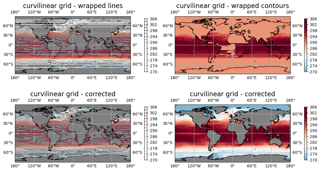
These kind of grids often makes it difficult to plot the data on its native
grid without remapping to a regular lonlat grid. For example, the
Matplotlib's contour and contourf functions wrap the contour lines around
most projections which looks streaky.
In this example we use the function z_masked_overlap() from htonchia at
https://github.com/SciTools/cartopy/issues/1421 to fix the wrapping problem.
The ncdump output of the input dataset:
netcdf MPI-ESM-LR_tos_20060101 {
dimensions:
x = 256 ;
y = 220 ;
nv4 = 4 ;
time = UNLIMITED ; // (1 currently)
nb2 = 2 ;
variables:
float lon(y, x) ;
lon:long_name = "longitude coordinate" ;
lon:units = "degrees_east" ;
lon:standard_name = "longitude" ;
lon:_CoordinateAxisType = "Lon" ;
lon:bounds = "lon_bnds" ;
float lon_bnds(y, x, nv4) ;
float lat(y, x) ;
lat:long_name = "latitude coordinate" ;
lat:units = "degrees_north" ;
lat:standard_name = "latitude" ;
lat:_CoordinateAxisType = "Lat" ;
lat:bounds = "lat_bnds" ;
float lat_bnds(y, x, nv4) ;
double time(time) ;
time:bounds = "time_bnds" ;
time:units = "days since 1850-01-01 00:00:00" ;
time:calendar = "proleptic_gregorian" ;
double time_bnds(time, nb2) ;
time_bnds:units = "days since 1850-01-01 00:00:00" ;
time_bnds:calendar = "proleptic_gregorian" ;
float tos(time, y, x) ;
tos:long_name = "Sea Surface Temperature" ;
tos:standard_name = "sea_surface_temperature" ;
tos:units = "K" ;
tos:coordinates = "lon lat" ;
tos:_FillValue = 1.e+20f ;
See also https://en.wikipedia.org/wiki/Curvilinear_coordinates
-------------------------------------------------------------------------------
2022 copyright DKRZ licensed under CC BY-NC-SA 4.0 <br>
(https://creativecommons.org/licenses/by-nc-sa/4.0/deed.en)
-------------------------------------------------------------------------------#
'''
import os
import xarray as xr
import numpy as np
import matplotlib.pyplot as plt
import cartopy.crs as ccrs
import cartopy.feature as cfeature
# Function z_masked_overlap() to prevent the line wrapping in contour plots
# The function z_masked_overlap was taken from
# https://github.com/SciTools/cartopy/issues/1421 from htonchia.
def z_masked_overlap(axe, X, Y, Z, source_projection=None):
"""
for data in projection axe.projection
find and mask the overlaps (more 1/2 the axe.projection range)
X, Y either the coordinates in axe.projection or longitudes latitudes
Z the data
operation one of 'pcorlor', 'pcolormesh', 'countour', 'countourf'
if source_projection is a geodetic CRS data is in geodetic coordinates
and should first be projected in axe.projection
X, Y are 2D same dimension as Z for contour and contourf
same dimension as Z or with an extra row and column for pcolor
and pcolormesh
return ptx, pty, Z
"""
if not hasattr(axe, 'projection'):
return X, Y, Z
if not isinstance(axe.projection, ccrs.Projection):
return X, Y, Z
if len(X.shape) != 2 or len(Y.shape) != 2:
return X, Y, Z
if (source_projection is not None and
isinstance(source_projection, ccrs.Geodetic)):
transformed_pts = axe.projection.transform_points(
source_projection, X, Y)
ptx, pty = transformed_pts[..., 0], transformed_pts[..., 1]
else:
ptx, pty = X, Y
with np.errstate(invalid='ignore'):
# diagonals have one less row and one less columns
diagonal0_lengths = np.hypot(
ptx[1:, 1:] - ptx[:-1, :-1],
pty[1:, 1:] - pty[:-1, :-1]
)
diagonal1_lengths = np.hypot(
ptx[1:, :-1] - ptx[:-1, 1:],
pty[1:, :-1] - pty[:-1, 1:]
)
to_mask = (
(diagonal0_lengths > (
abs(axe.projection.x_limits[1]
- axe.projection.x_limits[0])) / 2) |
np.isnan(diagonal0_lengths) |
(diagonal1_lengths > (
abs(axe.projection.x_limits[1]
- axe.projection.x_limits[0])) / 2) |
np.isnan(diagonal1_lengths)
)
# TODO check if we need to do something about surrounding vertices
# add one extra colum and row for contour and contourf
if (to_mask.shape[0] == Z.shape[0] - 1 and
to_mask.shape[1] == Z.shape[1] - 1):
to_mask_extended = np.zeros(Z.shape, dtype=bool)
to_mask_extended[:-1, :-1] = to_mask
to_mask_extended[-1, :] = to_mask_extended[-2, :]
to_mask_extended[:, -1] = to_mask_extended[:, -2]
to_mask = to_mask_extended
if np.any(to_mask):
Z_mask = getattr(Z, 'mask', None)
to_mask = to_mask if Z_mask is None else to_mask | Z_mask
Z = np.ma.masked_where(to_mask, Z)
return ptx, pty, Z
def main():
plt.switch_backend('agg')
#-- Open curvilinear dataset
fname = '../../data/MPI-ESM-LR_tos_20060101.nc'
ds = xr.open_dataset(fname)
var = ds.tos.isel(time=0)
lat = ds.lat
lon = ds.lon
#-- The coordinate arrays lat and lon are bounds, so the variable var should be
#-- the value inside those bounds. Therefore, the last value from the var array
#-- has to be removed.
var = var[:-1, :-1]
#-- Colormap
cmap = 'RdBu_r'
#-- Set vmin, vmax, and levels
vmin = 260.
vmax = 300.
levels = 20
#-- Create the figure
projection = ccrs.PlateCarree()
fig = plt.figure(figsize=(14, 8), constrained_layout=False)
#-- Define space for the four plots
gs = fig.add_gridspec(nrows=2, ncols=2, hspace=0, wspace=0.05)
#-- Generate the subplots
ax1 = plt.subplot(gs[0, 0], projection=projection)
ax2 = plt.subplot(gs[1, 0], projection=projection)
ax3 = plt.subplot(gs[0, 1], projection=projection)
ax4 = plt.subplot(gs[1, 1], projection=projection)
#-- Upper left plot
ax1.set_title('curvilinear grid - wrapped lines', fontsize=16)
ax1.set_global()
ax1.add_feature(cfeature.LAND, color='gray')
ax1.add_feature(cfeature.OCEAN, color='gray')
ax1.add_feature(cfeature.COASTLINE)
ax1.gridlines(draw_labels=True)
plot = ax1.contour(lon[:-1,:-1], lat[:-1,:-1], var,
cmap=cmap,
levels=levels,
vmin=vmin,
vmax=vmax,
linewidths=1.0)
plt.colorbar(plot, ax=ax1, shrink=0.6, pad=0.09)
#-- Compute the corrected data to prevent line wrapping. Use the dataset
#-- coordinates and variable.
X, Y, maskedZ = z_masked_overlap(ax1,
lon.data,
lat.data,
ds.tos.isel(time=0),
source_projection=ccrs.Geodetic())
#-- Lower left plot
ax2.set_global()
ax2.add_feature(cfeature.LAND, color='gray')
ax2.add_feature(cfeature.OCEAN, color='gray')
ax2.add_feature(cfeature.COASTLINE)
ax2.gridlines(draw_labels=True)
ax2.set_title('curvilinear grid - corrected', fontsize=16)
plot = ax2.contour(X, Y, maskedZ,
cmap=cmap,
levels=levels,
vmin=vmin,
vmax=vmax,
linewidths=1.0)
plt.colorbar(plot, ax=ax2, shrink=0.6, pad=0.09)
#-- Check if it works the same for contour fill.
#-- Display the incorrect and the corrected contour fill plot
#-- Upper right plot
ax3.set_title('curvilinear grid - wrapped contours', fontsize=16)
ax3.set_global()
ax3.add_feature(cfeature.LAND, color='gray')
ax3.add_feature(cfeature.OCEAN, color='gray')
ax3.add_feature(cfeature.COASTLINE)
ax3.gridlines(draw_labels=True)
plot = ax3.contourf(lon[:-1,:-1], lat[:-1,:-1], var,
cmap=cmap,
levels=levels,
vmin=vmin,
vmax=vmax)
plt.colorbar(plot, ax=ax3, shrink=0.6, pad=0.09)
#-- Use the already computed X, Y, maskedZ from above.
#-- lower right plot
ax4.set_global()
ax4.add_feature(cfeature.LAND, color='gray')
ax4.add_feature(cfeature.OCEAN, color='gray')
ax4.add_feature(cfeature.COASTLINE)
ax4.gridlines(draw_labels=True)
ax4.set_title('curvilinear grid - corrected', fontsize=16)
plot = ax4.contourf(X, Y, maskedZ,
cmap=cmap,
levels=levels,
vmin=vmin,
vmax=vmax)
plt.colorbar(plot, ax=ax4, shrink=0.6, pad=0.09)
plt.savefig('plot_curvilinear_contour_2x2_plots.png', bbox_inches='tight', dpi=100)
if __name__ == '__main__':
main()
Plot result: