Python slice-plot with topography#
Software requirements:
Python 3
numpy
xarray
matplotlib
cartopy
python-cdo
Example script#
slice_lon_height_topography.py
#!/usr/bin/env python
# coding: utf-8
'''
DKRZ example
Slices longitude versus height plus topography
Content
- read netCDF file
- create contour plot of the slice data
- generate topography data with CDO
- convert pressure levels to height
- add topography data to the slice plot
- save to PNG
-------------------------------------------------------------------------------
2022 copyright DKRZ licensed under CC BY-NC-SA 4.0 <br>
(https://creativecommons.org/licenses/by-nc-sa/4.0/deed.en)
-------------------------------------------------------------------------------
'''
#import os
import xarray as xr
import numpy as np
import matplotlib.pyplot as plt
import matplotlib.gridspec as gridspec
import cartopy.crs as ccrs
import cartopy.feature as cfeature
from cdo import Cdo
cdo = Cdo()
#------------------------------------------------------------------------------
# Function pressure_to_height(ds_flip)
#
# Function to convert the pressure coordinate in Pa to height in km.
# The data is in units 'Pa' and the topography in units 'm' that's why we
# convert the data to units 'm' too.
#------------------------------------------------------------------------------
def pressure_to_height(ds_flip):
"""
Transposed from the NCL procedure gsn_geop_hgt in
$NCARG_ROOT/ncl/lib/ncarg/nclscripts/csm/gsn_csm.ncl
'Returns geopotential height (in km) given array p (pressure in mb)
p must lie between 1013.25 mb and 2.54e-06 mb.
Algorithm is simply logarithmic interpolation from Standard
Atmosphere.
Intended to provide an ESTIMATE of geopotential height when
temperature and geopotential data are lacking.
Values above 85km were obtained from the COSPAR International
Reference Atmosphere: 1986 QB495 .A38 v.10 No.12 [FL]'
"""
pres = ds_flip.plev * 0.01
pres.attrs['units'] = 'hPa'
nsa = 53
# zsa in km
zsa = np.array([-0.3,
0.0, 0.5, 1.0, 1.5, 2.0, 2.5, 3.0,
3.5, 4.0, 4.5, 5.0, 5.5, 6.0, 6.5,
7.0, 7.5, 8.0, 8.5, 9.0, 9.5, 10.0,
11.0, 12.0, 13.0, 14.0, 15.0, 16.0, 17.0,
18.0, 19.0, 20.0, 25.0, 30.0, 35.0, 40.0, 45.0,
50.0, 60.0, 70.0, 80.0, 84.8, 87.7, 90.6,
93.3, 96.1, 97.5,100.4,104.9,
110.0,114.2,116.7,119.7])
# psa in hPa
psa = np.array([1050.,
1013.25, 954.61, 898.76, 845.59, 795.01, 746.91, 701.21,
657.80, 616.60, 577.52, 540.48, 505.39, 472.17, 440.75,
411.05, 382.99, 356.51, 331.54, 308.00, 285.84, 264.99,
226.99, 193.99, 165.79, 141.70, 121.11, 103.52, 88.497,
75.652, 64.674, 55.293, 25.492, 11.970, 5.746, 2.871, 1.491,
0.798, 0.220, 0.052, 0.010, 0.00485,0.00294,0.000178,
0.000108, 0.0000656, 0.0000511, 0.0000310, 0.0000146,
0.00000691, 0.00000419, 0.00000327, 0.00000254 ])
if (np.any(pres < min(psa)) or np.any(pres > max(psa))):
print("gsn_geop_hgt: Fatal: The pressure values do not fall between")
print(min(psa) + " mb and " + max(psa) + " mb.")
print("Error: Execution halted.")
npres = len(pres)
gph = np.zeros(npres,float)
for i in range(0,npres):
found = False
j = 0
while(not found and j <= nsa-2):
if((pres[i] <= psa[j]) and (pres[i] >= psa[j+1])):
gph[i] = zsa[j] + \
(zsa[j+1]-zsa[j])*np.log(psa[j]/pres[i])/np.log(psa[j]/psa[j+1])
found = True
j = j + 1
return gph
def main():
#--------------------------------------------------------------------------
# Plot 1
#
# Temperature
#
# The dataset CMIP5 atmos MPI-ESM-LR RCP 4.5 Air Temperature.
# Variable ta(time, plev, lat, lon)
#--------------------------------------------------------------------------
infile1 = '../../data/ta_Amon_t1.nc'
ds = xr.open_dataset(infile1)
ta = ds.ta
shapes = ds.ta.shape
# The longitudes in the plot from above are in range 0 to 360 deg, but we want
# them in range from -180 to 180 deg.
# Flip from 0-360 to -180-180 degrees.
ds_flip = ds.assign_coords(lon=(((ds.lon + 180) % 360) - 180)).sortby('lon')
# Extract the data at latitude 'sel_lat' for the first time step.
sel_lat = 47.
data_flip = ds_flip.ta.isel(time=0).sel(lat=sel_lat, method='nearest')
# Create the plot with the flipped data and longitudes as well as invert the y-axis.
fig, ax = plt.subplots(figsize=(16,8))
plt.contourf(data_flip.lon.values, ds.plev, data_flip, cmap='viridis')
ax.invert_yaxis()
ax.set_xlabel('longitude')
ax.set_ylabel('pressure level')
ax.set_title('Air Temperature at lat '+str(sel_lat)+'$^\circ$N t=0')
plt.savefig('plot_slice_02.png', bbox_inches='tight')
#--------------------------------------------------------------------------
# Plot 2
#
# Temperture plus topography and map
#
# CDO provides the operator 'topo' to generate the global topography data in
# meters. During the computation the data will be interpolated to the same
# grid as the input data file.
#
# The input string for the remapbil operator can be constructed by the stored
# shapes of the data.
#--------------------------------------------------------------------------
grid = 'r'+str(shapes[3])+'x'+str(shapes[2])
cdo.remapbil(grid, input='-topo', output='topo.nc', options='-O -f nc')
# Read the topography dataset.
ds_topo = xr.open_dataset('topo.nc')
# Flip the longitudes and the data from 0-360 to -180-180.
ds_topo_flip = ds_topo.assign_coords(lon=(((ds_topo.lon + 180) % 360) - 180)).sortby('lon')
# Extract the data at latitude 'sel_lat'.
topo = ds_topo_flip.topo.sel(lat=sel_lat, method='nearest')
#--------------------------------------------------------------------------
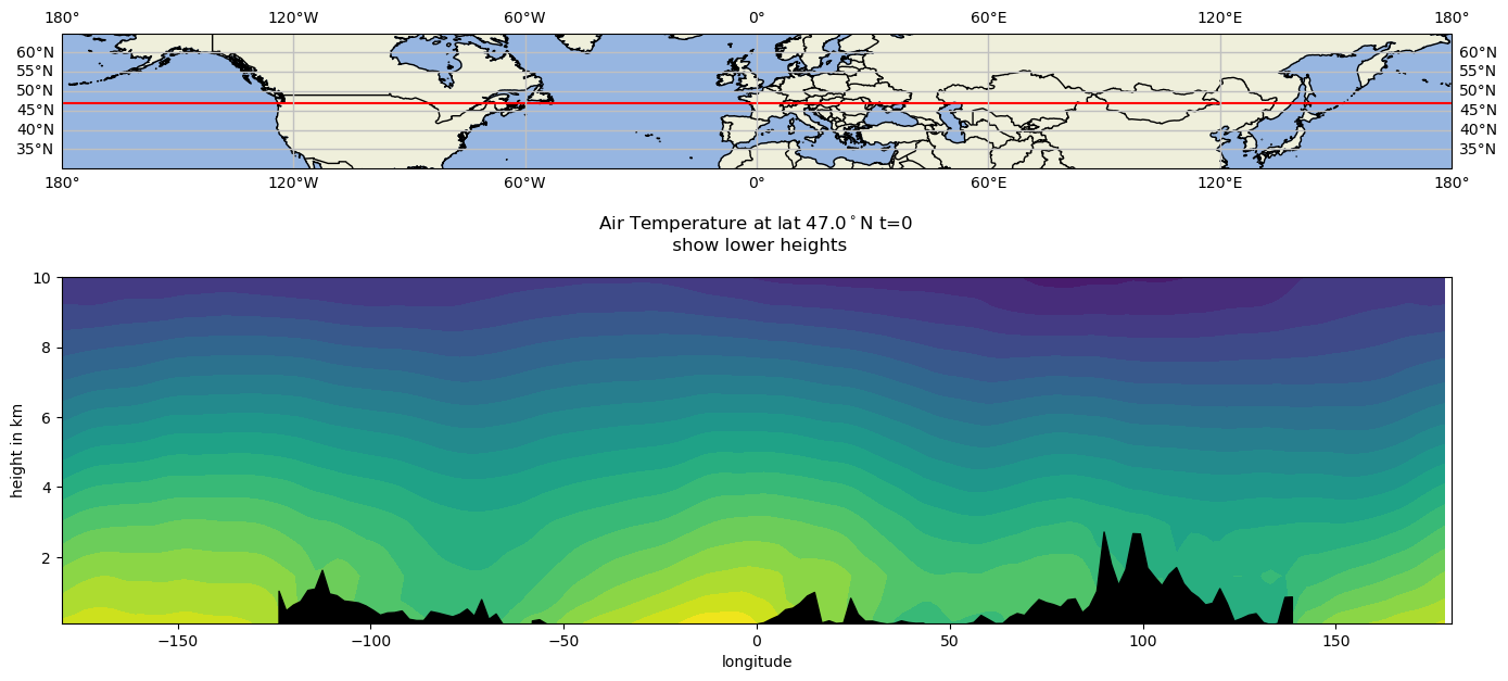
# Plot slice and topography in same figure, and the map above
# Extract the data at latitude 'sel_lat' of the first time step.
data_flip = ds_flip.ta.isel(time=0).sel(lat=sel_lat, method='nearest')
#-- Convert the pressure levels (Pa) to height (km).
height = pressure_to_height(ds_flip)
# Now, we draw the contours of the variable 'ta' but we use the height instead
# of the pressure levels. Afterwards, the topography data is drawn as a
# black contour. We use the 'twinx()' method to add the topography plot to the
# contour plot. This allows us to set the right axis labels which in this case
# is the same as the left one. To see the topography better we show only a
# small range of the y-axis.
projection = ccrs.PlateCarree()
maxy = 10.
miny = height.min()
fig = plt.figure(figsize=(16, 8))
gs = gridspec.GridSpec(nrows=2, ncols=1, left=0.1, right = 0.9,
bottom=0.1, top=0.9, hspace=0.01)
#-- small map
ax1 = plt.subplot(gs[0, 0], projection=projection)
ax1.add_feature(cfeature.LAND)
ax1.add_feature(cfeature.OCEAN)
ax1.add_feature(cfeature.BORDERS)
ax1.add_feature(cfeature.COASTLINE)
ax1.set_extent([-180., 180., 30., 65.], crs=ccrs.PlateCarree())
ax1.plot([-180., 180.], [47., 47.], color='red', transform=ccrs.PlateCarree())
ax1.gridlines(draw_labels=True,
linewidth=1,
color='silver',
crs=ccrs.PlateCarree())
#-- plot slice with topography
ax2 = plt.subplot(gs[1, 0], sharex=ax1)
ax2.contourf(data_flip.lon.values, height, data_flip, levels=20, cmap='viridis')
ax2.set_xlabel('longitude')
ax2.set_ylabel('height in km')
ax2.set_ylim(miny, maxy)
ax2.fill_between(data_flip.lon.values, topo/1000, where=topo>=0, color='black')
tx = plt.title('Air Temperature at lat '+str(sel_lat)+'$^\circ$N t=0 \n show lower heights', y=1.05)
plt.savefig('plot_slice_03.png', bbox_inches='tight')
if __name__ == '__main__':
main()
Plot result: