Python: FESOM: plot the cells of the unstructured data#
Description
If you want to display the unstructured data of an FESOM model output in a map, then in most cases this grid is remapped to a regular grid. However, if we want to display the data on the original grid, we must first define the cells defined by the cell vertices as polygons. Then the data values can be colored, this is done by assigning the colors with which the cells are then filled.
Content
Read FESOM data
Extract a subregion
Generate the Polygons from the vertices
Symmetric value range (vmin,vmax) - Create the colormap - Compute the norm - Get the colors for each cell - Plotting
Asymmetric value range (vmin,vmax) - Define colormap midpoint and cut off outlaying colors - Compute the norm - Plotting
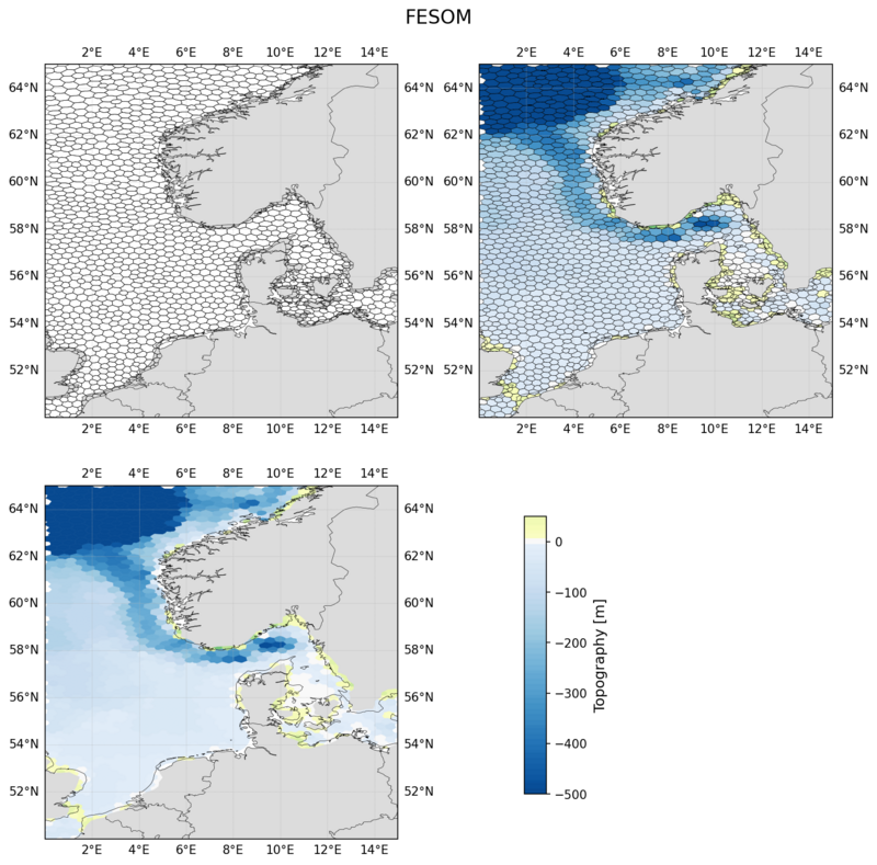
Plotting: conla cell bounds, data and cell bounds, and data only
Software requirements
Python 3
numpy
xarray
matplotlib
cartopy
shapely
geopandas
Example script#
fesom_unstructured_grid.py
#!/usr/bin/env python
# coding: utf-8
#------------------------------------------------------------------------------
#
# FESOM: plot the cells of the unstructured data
#
#------------------------------------------------------------------------------
# 2025 copyright DKRZ licensed under CC BY-NC-SA 4.0
#                (https://creativecommons.org/licenses/by-nc-sa/4.0/deed.en)
#------------------------------------------------------------------------------
#
# If you want to display the unstructured data of an FESOM model output in a
# map, then in most cases this grid is remapped to a regular grid. However, if
#  we want to display the data on the original grid, we must first define the
# cells defined by the cell vertices as polygons. Then the data values can be
# colored, this is done by assigning the colors with which the cells are then
# filled.
#
# Content
#
# - Read FESOM data
# - Extract a subregion
# - Generate the Polygons from the vertices
# - Symmetric value range (vmin,vmax)
#   - Create the colormap
#   - Compute the norm
#   - Get the colors for each cell
#   - Plotting
# - Asymmetric value range (vmin,vmax)
#   - Define colormap midpoint and cut off outlaying colors
#   - Compute the norm
#   - Plotting
# - Plotting: conla cell bounds, data and cell bounds, and data only
#
#
# FESOM
#
# - Home:https://fesom.de/cmip6/work-with-awi-cm-unstructured-data/
# - How to work with Fesom2 data: https://fesom.de/cmip6/work-with-awi-cm-unstructured-data/
#
#
# Data
#
# The links to the example data are taken from **PyFESOM2**: https://github.com/FESOM/pyfesom2/tree/main
#
# - 2D  https://swift.dkrz.de/v1/dkrz_0262ea1f00e34439850f3f1d71817205/FESOM/tos_Omon_AWI-ESM-1-1-LR_historical_r1i1p1f1_gn_185001-185012.nc
#
# - 3D  https://swift.dkrz.de/v1/dkrz_0262ea1f00e34439850f3f1d71817205/FESOM/thetao_Omon_AWI-ESM-1-1-LR_historical_r1i1p1f1_gn_185001-185012.nc
#
# Convert unstructured grid to regular lon/lat grid
#
# If you prefer to work with regular grids, the FESOM data can be remapped as
# follows:
#
#     cdo genycon,global_1 <inputpath>/<inputfilename> <outputpath>/<weightsfilename>
#     cdo remap,global_1,<outputpath>/<weightsfilename> <inputpath>/<inputfilename> \
#                                                       <outputpath>/<outputfilename>
#------------------------------------------------------------------------------
import os
import xarray as xr
import numpy as np

import geopandas as gpd

import matplotlib.pyplot as plt
import matplotlib.colors as mcolors
import matplotlib.colorbar as colorbar

import cartopy.crs as ccrs
import cartopy.feature as cfeature

from shapely.geometry import Polygon

#plt.switch_backend('agg')

#-- Read FESOM data
ds = xr.open_dataset(os.environ['HOME']+'/data/FESOM/fesom_topo_exact.nc')

#-- Extract a subregion
lonmin, lonmax = 0., 15.
latmin, latmax = 50., 65.

ds_subset = ds.where((ds.lon > lonmin) &
                     (ds.lon < lonmax ) &
                     (ds.lat > latmin ) &
                     (ds.lat < latmax ), drop=True)

#-- Retrieve the number of cells and vertices for the subregion.
for key,value in ds_subset.sizes.items():
    locals()[key] = value

print(f'subregion: ncells = {ncells}   nv = {nv}')

#--------------------------------------------
#-- Generate the Polygons from the vertices
#--------------------------------------------
#-- Generate the list of (x,y) pairs for each cell.
polygon_geometries = [[ list(t) for t in zip(ds_subset.lon_vertices[i,:].values.tolist(),
                                             ds_subset.lat_vertices[i,:].values.tolist()) ] for i in range(ncells) ]

#-- Generate the Polygons from the polygon_geometries.
polygons = []
for i in range(len(polygon_geometries)):
    p = Polygon(polygon_geometries[i][:])
    polygons.append(p)

#-- We can use GeoPandas GeoDataFrame and the GeoSeries of the polygons to
#-- generate a GeoDataFrame. This creates the needed geometry data that we can
#-- now merge with the topo, lon, and lat data from the df DataFrame.
geoseries = gpd.GeoDataFrame(gpd.GeoSeries(polygons), columns=['geometry'])

#--------------------------------------
#-- Symmetric value range (vmin,vmax)
#--------------------------------------
vmin, vmax = -500, 500

#-- Create the colormap
inc = 10
levels = np.arange(vmin, vmax, inc, dtype='float')
llen = levels.shape[0]

blues    = plt.cm.Blues_r(np.linspace(0.1, 0.9, int(llen/2)))
white    = plt.cm.Greys_r(np.linspace(0.95, 1., 1))
greens   = plt.cm.YlGn(np.linspace(0.1, 0.9, int(llen/2)))
col_list = np.vstack((blues, white, greens))
N        = col_list.shape[0]

cmap = mcolors.LinearSegmentedColormap.from_list('topo_map', col_list, N=N)

#-- Compute the norm
norm = mcolors.Normalize(vmin=vmin, vmax=vmax)

#-- Get the colors for each cell
colors = []

idata   = ncells
jcolors = levels.shape[0]

for i in range(0, idata, 1):
    for j in range(0, jcolors-1, 1):
        if ds_subset.topo[i] < levels[0]:
            colors.append(col_list[0])
            break
        elif ds_subset.topo[i] >= levels[-1]:
            colors.append(col_list[-1])
            break
        elif (ds_subset.topo[i] > levels[j]) and (ds_subset.topo[i] <= levels[j+1]):
            colors.append(col_list[j+1])
            break

#--------------
#-- Plotting
#--------------
fig, ax = plt.subplots(figsize=(6,5), subplot_kw=dict(projection=ccrs.PlateCarree()))

ax.set_extent([lonmin, lonmax, latmin, latmax], crs=ccrs.PlateCarree())
ax.add_feature(cfeature.LAND.with_scale('10m'), color='gainsboro')
ax.add_feature(cfeature.BORDERS.with_scale('10m'), linewidth=0.3)
ax.add_feature(cfeature.COASTLINE.with_scale('10m'), linewidth=0.3, zorder=6);
ax.gridlines(draw_labels=True, lw=0.4, ls=':')

for i in range(ncells):
    pgon = geoseries['geometry'][i]
    ax.add_geometries([pgon], crs=ccrs.PlateCarree(),
                      edgecolor=colors[i],
                      facecolor=colors[i])
#-- add colorbar
x,y,w,h = 0.93, 0.2, 0.2, 0.6
cax = fig.add_axes([x, y, w/14, h-0.03], autoscalex_on=True)
cbar = colorbar.Colorbar(cax, orientation='vertical', cmap=cmap, norm=norm, alpha=1)
cbar.set_label(label='Topography [m]', loc='center', labelpad=5, size=12);

plt.savefig('plot_FESOM_subregion_1.png', bbox_inches='tight',dpi=150)

plt.show()

#---------------------------------------
#-- Asymmetric value range (vmin,vmax)
#---------------------------------------
#-- Therefore we only need to compute the norm in a different way.
vmin2, vmax2 = -500., 50.

#-- Define colormap midpoint and cut off outlaying colors
#--
#-- The next example demonstrates the use of a pre-defined colormap with a user
#-- defined subclass of the `matplotlib.colors.Normalize` class to generate the
#-- plot and it's colorbar cutting off outlaying colors.
#--
#-- Based on an example from _Stack Overflow_: <br>
#-- https://stackoverflow.com/questions/55665167/asymmetric-color-bar-with-fair-diverging-color-map <br>
#-- https://stackoverflow.com/questions/7404116/defining-the-midpoint-of-a-colormap-in-matplotlib <br>

#-- subclassing cm.Normalize
class MidpointNormalize(mcolors.Normalize):
    def __init__(self, vmin=None, vmax=None, midpoint=None, clip=False):
        self.midpoint = midpoint
        mcolors.Normalize.__init__(self, vmin, vmax, clip)
    def __call__(self, value, clip=None):
        v_ext = np.max( [ np.abs(self.vmin), np.abs(self.vmax) ] )
        x, y = [-v_ext, self.midpoint, v_ext], [0, 0.5, 1]
        return np.ma.masked_array(np.interp(value, x, y))

#-- Compute the norm
norm2 = MidpointNormalize(midpoint=0, vmin=vmin2, vmax=vmax2)

#-------------
#-- Plotting
#-------------
draw_cell_bounds = 'both'   # 'only', 'both', 'none'

fig, ax = plt.subplots(figsize=(6,5), subplot_kw=dict(projection=ccrs.PlateCarree()))

ax.set_extent([lonmin, lonmax, latmin, latmax], crs=ccrs.PlateCarree())
ax.add_feature(cfeature.LAND.with_scale('10m'), color='gainsboro')
ax.add_feature(cfeature.BORDERS.with_scale('10m'), linewidth=0.3)
ax.add_feature(cfeature.COASTLINE.with_scale('10m'), linewidth=0.3, zorder=6);
ax.gridlines(draw_labels=True, lw=0.4, ls=':')

for i in range(ncells):
    pgon = geoseries['geometry'][i]

    if draw_cell_bounds == 'only':
        edgecolor = 'k'
        facecolor = 'None'
    elif draw_cell_bounds == 'both':
        edgecolor = 'k'
        facecolor = colors[i]
    else:
        edgecolor = colors[i],
        facecolor = colors[i]

    kwargs = dict(edgecolor=edgecolor, facecolor=facecolor, linewidth=0.3)

    ax.add_geometries([pgon], crs=ccrs.PlateCarree(), **kwargs)

#-- add colorbar
if draw_cell_bounds != 'only':
    x,y,w,h = 0.93, 0.2, 0.2, 0.6
    cax = fig.add_axes([x, y, w/14, h-0.03], autoscalex_on=True)
    cbar = colorbar.Colorbar(cax, orientation='vertical', cmap=cmap, norm=norm2, alpha=1)
    cbar.set_label(label='Topography [m]', loc='center', labelpad=5, size=12);

plt.savefig('plot_FESOM_subregion_2.png', bbox_inches='tight',dpi=150)

plt.show()

#--------------------------------------------------------------
#-- Plotting:
#--    only cells bounds, data and cell bounds, and data only
#--------------------------------------------------------------
fig, axes = plt.subplots(nrows=2, ncols=2, figsize=(10,10),
                         layout='constrained',
                         subplot_kw=dict(projection=ccrs.PlateCarree()))

ctypes = ['only', 'both', 'none']

for j, ax in enumerate(axes.flat):
    if j < axes.size-1:
        ax.set_extent([lonmin, lonmax, latmin, latmax], crs=ccrs.PlateCarree())
        ax.add_feature(cfeature.LAND.with_scale('10m'), color='gainsboro')
        ax.add_feature(cfeature.BORDERS.with_scale('10m'), linewidth=0.3)
        ax.add_feature(cfeature.COASTLINE.with_scale('10m'), linewidth=0.3, zorder=6);
        ax.gridlines(draw_labels=True, lw=0.4, ls=':')

        if j < axes.size-1: draw_cell_bounds = ctypes[j]

        for i in range(ncells):
            #pgon = df_all.geometry[i]
            pgon = geoseries['geometry'][i]

            if draw_cell_bounds == 'only':
                edgecolor = 'k'
                facecolor = 'None'
            elif draw_cell_bounds == 'both':
                edgecolor = 'k'
                facecolor = colors[i]
            else:
                edgecolor = colors[i],
                facecolor = colors[i]

            kwargs = dict(edgecolor=edgecolor, facecolor=facecolor, linewidth=0.3)

            ax.add_geometries([pgon], crs=ccrs.PlateCarree(), **kwargs)
    else:
        #-- add colorbar
        ax.set_visible(False)
        bbox = ax.get_position()
        x, y, w, h = bbox.x0, bbox.y0, bbox.width, bbox.height
        cax = fig.add_axes([x+0.05, y-0.02, w/14, h-0.03], autoscalex_on=True)
        cbar = colorbar.Colorbar(cax, orientation='vertical', cmap=cmap, norm=norm2, alpha=1)
        cbar.set_label(label='Topography [m]', loc='center', labelpad=5, size=12);

fig.suptitle('FESOM', fontsize=16)
plt.savefig('plot_FESOM_subregion_3.png', bbox_inches='tight', dpi=150)

plt.show()
Plot result#