Python: hillshading#
Description
This example shows how to work with ETOPO topography data or with the NaturalEarthRelief images. It highlights various methods such as ax.imshow() and ax.pcolormesh(), before moving to the actual goal, the data overlay plot.
The topography can be ‘hill shaded’ with Matplotlib’s LightSource methods. This allows us to use the result in a plot that overlays data with transparency
Content
Read topography data
Choose a map projection
Create a colormap
Display topography data
Matplotlib’s LightSource
Plotting - With ax.imshow() - With ax.pcolormesh()
Overlay example data on the topography
Only briefly mentioned - Display coarse standard NaturalEarthRelief image - Display high resolution NaturalEarthRelief image
Software requirements
Python 3
numpy
xarray
matplotlib
cartopy
Example script#
hillshading_global_topography.py
#!/usr/bin/env python
# coding: utf-8
#------------------------------------------------------------------------------
#
# DKRZ Python Course for Geoscientists - Vis A11
#
# Relief shading
#
#------------------------------------------------------------------------------
# 2025 copyright DKRZ licensed under CC BY-NC-ND 4.0
# (https://creativecommons.org/licenses/by-nc-nd/4.0/deed.en)
#------------------------------------------------------------------------------
#
# This notebook shows how to work with ETOPO topography data or with the
# NaturalEarthRelief images. It highlights various methods such as ax.imshow()
# and ax.pcolormesh(), before moving to the actual goal, the data overlay plot.
#
# The topography can be 'hill shaded' with Matplotlib's LightSource methods.
# This allows us to use the result in a plot that overlays data with transparency
# on it.
#
# Content
#
# 1. Read topography data
# 2. Choose a map projection
# 3. Create a colormap
# 4. Display topography data
# 5. Matplotlib's LightSource
# 6. Plotting
# 1. With `ax.imshow()`
# 2. With `ax.pcolormesh()`
# 7. Overlay example data on the topography
# 8. Only briefly mentioned
# 3. Display coarse standard NaturalEarthRelief image
# 4. Display high resolution NaturalEarthRelief image
#
# ETOPO Global Relief Model: https://www.ncei.noaa.gov/products/etopo-global-relief-model
#
# NaturalEarth shaded relief: https://www.naturalearthdata.com/
#
# Matplotlib's hillshading: https://matplotlib.org/stable/gallery/specialty_plots/topographic_hillshading.html#sphx-glr-gallery-specialty-plots-topographic-hillshading-py
#
#------------------------------------------------------------------------------
import os
import xarray as xr
import numpy as np
import matplotlib.pyplot as plt
import matplotlib.colors as mcolors
from matplotlib.colors import LightSource
import matplotlib.cm as mcm
import matplotlib.colorbar as mcolorbar
import cartopy.crs as ccrs
import cartopy.feature as cfeature
#-- Read Topography data
#
# We have already downloaded the data from the NOAA website (see link above)
# and converted the data into global 0.1° x 0.1° grid resolution with CDO.
topo_file = os.environ['HOME']+'/data/ETOPO/topo_global_0.1_cdo.nc'
#-- Use Xarray to open and read the topography data.
ds = xr.open_dataset(topo_file)
ds = ds.isel(lat=slice(None, None, -1)) #-- reverse latitude
#print(ds)
#-- Read the variable 'topo'.
topo = ds.topo.data
print(topo.min(), topo.max())
print(topo.shape)
#-- Read the latitude and longitude data
lon = ds.lon.data
lat = ds.lat.data
#-- Get the coordinate increments
dx = ds.lon[1].data - ds.lon[0].data
dy = ds.lat[1].data - ds.lat[0].data
#-- Choose a map projection
proj = ccrs.PlateCarree()
#-- Create a colormap for the topography
colors_blues = plt.cm.Blues_r(np.linspace(0.1, 0.9, 24))
colors_greens = plt.cm.summer_r(np.linspace(0.3, 1., 20))
colors_browns = plt.cm.pink(np.linspace(0.2, 0.6, 3))
colors_white = plt.cm.Greys_r(np.linspace(0.95, 1., 1))
#-- Attach the individual color components to a single color array
all_colors = np.vstack((colors_blues, colors_greens, colors_browns, colors_white))
topo_cmap = mcolors.LinearSegmentedColormap.from_list('topo_map', all_colors)
#-- Let's help the Netherlands not to drown by setting vcenter=5
divnorm = mcolors.TwoSlopeNorm(vmin=-6000., vcenter=5, vmax=6000)
#print(topo_cmap)
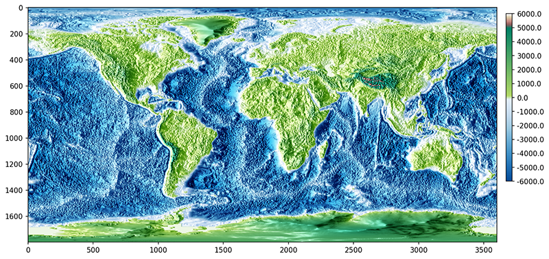
#-- Display topography data
fig, ax = plt.subplots(figsize=(12,6), subplot_kw=dict(projection=proj))
plot = ax.pcolormesh(lon, lat, topo,
cmap=topo_cmap,
norm=divnorm,
transform=proj)
cbar = plt.colorbar(plot, shrink=0.5)
ax.coastlines(lw=0.4)
ax.gridlines(draw_labels=True, color='None')
plt.savefig('plot_hillshading_topography_0.png', bbox_inches='tight', facecolor='white', dpi=150)
#-- Matplotlib's LightSource
#
# In this second example we use the Matplotlib LightSource method to generate
# the shaded relief of the topography data. The azimuth and elevation of the
# light source is taken as input parameters.
#
# See https://matplotlib.org/stable/api/_as_gen/matplotlib.colors.LightSource.html#matplotlib.colors.LightSource
#
# Shade from the west, with the sun 30° from horizontal.
ls = LightSource(azdeg=270, altdeg=30)
# The 'shade' method is used here to generate an (m,n,4)-array of zeros and ones
# to be used in the 'shade_rgb' helper method.
#
# Combine colormapped data values with an illumination intensity map (aka
# 'hillshade') of the values - see https://matplotlib.org/stable/api/_as_gen/matplotlib.colors.LightSource.html#matplotlib.colors.LightSource.shade
rgb = ls.shade(topo,
cmap=topo_cmap,
norm=divnorm,
blend_mode='soft',
vert_exag=0.5,
dx=lon,
dy=lat)
#print(rgb.shape)
# Use the helper function 'shade_rgb' to adjust the colors of the rgb-array
# from above to be able to simulate a shaded relief, read
# https://matplotlib.org/stable/api/_as_gen/matplotlib.colors.LightSource.html#matplotlib.colors.LightSource.shade_rgb
data_hillshade = ls.shade_rgb(rgb,
topo,
blend_mode='soft',
vert_exag=0.5,
dx=lon,
dy=lat)
#print(data_hillshade.shape)
#print(topo.shape)
#-- Plotting
#
# To display the topography data with the shading computed above we can use two
# different approaches, with 'ax.imshow()' or with 'ax.pcolormesh()'.
#
# With 'ax.imshow()'
#
# In the first plotting example we use the _data_hillshade_ we have computed
# above and display it with the 'ax.imshow()' method.
#from mpl_toolkits.axes_grid1 import make_axes_locatable
fig,ax = plt.subplots(figsize=(12,6))
plot = ax.imshow(data_hillshade, interpolation='bilinear')
#-- add custom colorbar
cax = fig.add_axes([ax.get_position().x1+0.015,
ax.get_position().y0+0.2,
0.01, #-- width
ax.get_position().height/1.4])
cbar_ticks = np.arange(divnorm.vmin, divnorm.vmax+100, 100)
cbar_labels = [str(x) for x in cbar_ticks]
cbar = mcolorbar.Colorbar(cax,
cmap=topo_cmap,
norm=divnorm,
ticks=cbar_ticks,
orientation = 'vertical')
cbar.set_ticks(cbar_ticks[::10], labels=cbar_labels[::10])
plt.savefig('plot_hillshading_topography_1.png', bbox_inches='tight', facecolor='white', dpi=150)
# With 'ax.pcolormesh()'
#
# The next example uses the same LightSource arrays here we use 'ax.pcolormesh'
# instead of 'ax.imshow' that allows us to use a map projection, add coastlines
# and draw the correct axes labels.
fig, ax = plt.subplots(figsize=(12,6), subplot_kw=dict(projection=proj))
ls = LightSource(azdeg=315, altdeg=45)
ax.pcolormesh(lon, lat, data_hillshade,
cmap=topo_cmap,
norm=divnorm,
transform=ccrs.PlateCarree())
ax.gridlines(draw_labels=True, color='None')
ax.coastlines(color='red')
#-- add custom colorbar
cax = fig.add_axes([ax.get_position().x1+0.04,
ax.get_position().y0+0.05,
0.01,
ax.get_position().height/1.4])
cbar_ticks = np.arange(divnorm.vmin, divnorm.vmax+100, 100)
cbar_labels = [str(x) for x in cbar_ticks]
cbar = mcolorbar.Colorbar(cax,
cmap=topo_cmap,
norm=divnorm,
ticks=cbar_ticks,
orientation = 'vertical')
cbar.set_ticks(cbar_ticks[::10], labels=cbar_labels[::10])
plt.savefig('plot_hillshading_topography_2.png',
bbox_inches='tight', facecolor='white', dpi=150)
#------------------------------------------------------------------------------
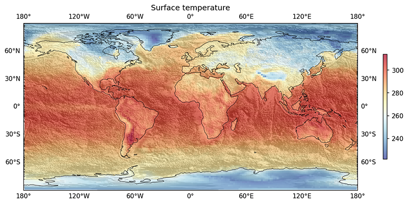
# Overlay example data on the topography
#
# In the following we show an example of a plot that displays surface temperature
# data on top of the ETOPO5 topography data.
#
# First, we need to generate the LightSource object with a grey colormap for
# the background topography.
#------------------------------------------------------------------------------
greys = plt.cm.Greys_r(np.linspace(0.3, 1., 64))
topo_greys = mcolors.LinearSegmentedColormap.from_list('topo_greys', greys)
rgb2 = ls.shade(topo,
cmap=topo_greys,
norm=divnorm,
blend_mode='soft',
vert_exag=0.5,
dx=lon,
dy=lat)
data_hillshade2 = ls.shade_rgb(rgb2,
topo,
blend_mode='soft',
vert_exag = 0.5,
dx=lon,
dy=lat)
#-- Read the example surface temperature data
data_file = os.environ['HOME'] + '/data/rectilinear_grid_2D.nc'
ds = xr.open_dataset(data_file)
var = ds.tsurf.isel(time=0)
#-- Create the overlay plot
#
# Both the topography and the data are drawn slightly transparent, on the one
# hand to make the gray tones of the topography appear softer, and on the other
# hand to allow the topography to shine through at all.
fig, ax = plt.subplots(figsize=(12,6), subplot_kw=dict(projection=proj))
ax.tick_params(right= True, top= False, left= True, bottom= True)
ax.pcolormesh(lon, lat, data_hillshade2,
cmap=topo_greys,
norm=divnorm,
alpha=0.5, # use transparency for lighter greys
transform=ccrs.PlateCarree())
ax.set_title('Surface temperature')
plot_var = ax.pcolormesh(var.lon, var.lat, var,
cmap='RdYlBu_r',
alpha=0.7, # set transparency
transform=ccrs.PlateCarree())
cbar = plt.colorbar(plot_var, orientation='vertical',
shrink=0.5, pad=0.06, aspect=25)
ax.gridlines(draw_labels=True, color='None')
ax.coastlines(color='black', lw=0.5)
plt.savefig('plot_hillshading_topography_overlayed_temperature.png',
bbox_inches='tight', facecolor='white', dpi=150)
#------------------------------------------------------------------------------
# Only briefly mentioned
#
# Display coarse standard NaturalEarthRelief image
#
# The standard image file is stored in your default Python environment
# installation folder, e.g. 'lib/python3.12/site-packages/cartopy/data/raster/natural_earth/'.
#------------------------------------------------------------------------------
#-- With 'ax.stock_img()'
fig, ax = plt.subplots(figsize=(10,5), subplot_kw=dict(projection=proj))
ax.set_extent([-180,180,-90,90], crs=ccrs.PlateCarree())
#-- display a coarse NaturalEarth shaded relief image in the background
ax.stock_img()
ax.set_title('ax.stock_image(): NaturalEarth shaded relief', y=1.1)
ax.coastlines(lw=0.4)
plt.savefig('plot_hillshading_topography_ner1.png',
bbox_inches='tight', facecolor='white')
#-- Display high resolution NaturalEarthRelief image
#
# With 'ax.background_img'
#
# Display an already downloaded high resolution NaturalEarthRelief image in the
# background.
#
# Have a look at the example script 'Python high resolution background image'
# at https://docs.dkrz.de/doc/visualization/sw/python/source_code/python-matplotlib-example-high-resolution-background-image-plot.html#dkrz-python-matplotlib-example-high-resolution-background-image-plot
# to learn more about the work with downloaded background images in Matplotlib.
#
# Path to CARTOPY_USER_BACKGROUNDS environment variable:
#-- save default path
def_path_cub = os.environ.get('CARTOPY_USER_BACKGROUNDS')
#-- set environment variable CARTOPY_USER_BACKGROUNDS
os.environ['CARTOPY_USER_BACKGROUNDS'] = '../../../Backgrounds/'
#print(f'CARTOPY_USER_BACKGROUNDS\ndefault: {def_path_cub}\nnew: {os.environ.get('CARTOPY_USER_BACKGROUNDS')}')
#-- plotting
fig, ax = plt.subplots(figsize=(10,5), subplot_kw=dict(projection=proj))
#-- display a high-res NaturalEarth shaded relief image in the background
ax.background_img(name='NaturalEarthRelief', resolution='high')
ax.coastlines(resolution='10m', lw=0.4)
gl = ax.gridlines(draw_labels=True)
gl.xlines = False
gl.ylines = False
gl.left_labels = False
ax.set_title('ax.background_img() - NaturalEarth high resolution')
plt.savefig('plot_hillshading_topography_ner2.png',
bbox_inches='tight', facecolor='white')
Plot result#