Python latitude versus height#
Software requirements:
Python 3
numpy
xarray
matplotlib
Example script#
This Python script is the equivalent of an NCL script from Marco Giorgetta and Renate Brokopf from Max-Planck-Institut für Meteorologie, Hamburg, Germany. Thank you for providing the NCL script and the data.
generate_lat_vs_height_hus.py
#!/usr/bin/env python
# coding: utf-8
'''
DKRZ example
Zonal mean lat vs. height specific humidity
This Python script is the equivalent of an NCL script from Marco Giorgetta
and Renate Brokopf from Max-Planck-Institut für Meteorologie, Hamburg,
Germany. Thank you for providing the NCL script and the data.
Generate two plot
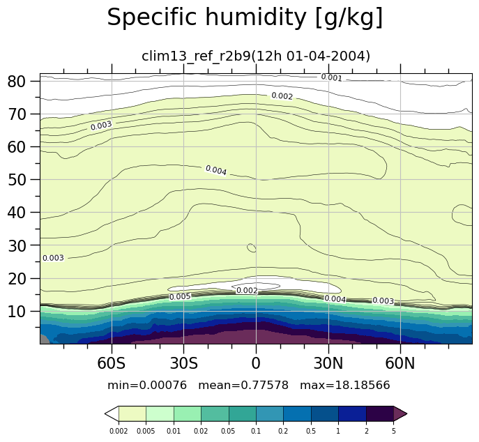
1. Specfic humidity code133 zonal CMOR: hus
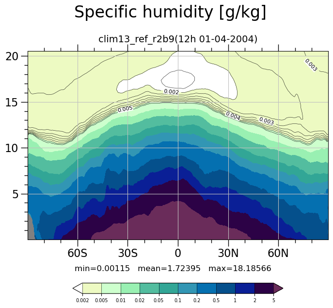
2. Specfic humidity code133 zonal CMOR: hus - code 133 up to 20 km
NCL Colormaps
If we use an NCL colormap, then the RGB/RGBA values still have to be
prepared for Matplotlib.
- either copy the colormap from NCARG_ROOT/lib/ncarg/colormaps folder to
a local folder or use the colormap directly from the NCL installation
environment
- an unknown number of header lines has to be skip
- the RGB values can be in range 0-255 or 0.0-1.0 but Matplotlib accepts
only range 0.0-1.0
- use the colors rgb[1:,:] for the cmap
- define the under, over, and bad colors explicitly
Content
- read netCDF file
- read NCL colormap
- save to PNG
-------------------------------------------------------------------------------
2024 copyright DKRZ licensed under CC BY-NC-SA 4.0 <br>
(https://creativecommons.org/licenses/by-nc-sa/4.0/deed.en)
-------------------------------------------------------------------------------
'''
import os
import xarray as xr
import numpy as np
import matplotlib.pyplot as plt
from matplotlib.ticker import MultipleLocator
import matplotlib.colors as mcolors
# Function get_NCL_colormap
def get_NCL_colormap(colormap_file, extend='None'):
'''Read an NCL RGB colormap file and convert it to a Matplotlib colormap object.
Parameter:
colormap_file path to NCL RGB colormap file.
extend use NCL behavior of color handling for the colorbar 'under'
and 'over' colors. 'None' or 'ncl', default 'None'
Description:
For example the NCL colormap name "ncl_default" points to the
colormap file $NCARG_ROOT/lib/ncarg/colormaps/ncl_default.rgb
Returns a colormap object.
'''
from matplotlib.colors import ListedColormap
#-- read the NCL colormap RGB file
cfile = os.path.split(colormap_file)[1]
if os.path.isfile(colormap_file) == False:
if 'NCARG_ROOT' in os.environ:
cpath = os.environ['NCARG_ROOT']+'/lib/ncarg/colormaps/'
if os.path.isfile(cpath + cfile): colormap_file = cpath + cfile
else:
import errno
raise FileNotFoundError(errno.ENOENT, os.strerror(errno.ENOENT), colormap_file)
with open(colormap_file) as f:
lines = f.read().splitlines()
#-- skip all possible header lines
tmp = [ x for x in lines if 'ncolors' not in x ]
tmp = [ x for x in tmp if '#' not in x ]
tmp = [ x for x in tmp if ';' not in x ]
tmp = [ x for x in tmp if x != '']
#-- get the RGB values
i = 0
for l in tmp:
new_array = np.array(l.split()).astype(float)
if i == 0:
color_list = new_array
else:
color_list = np.vstack((color_list, new_array))
i += 1
#-- make sure that the RGB values are within range 0 to 1
if (color_list > 1.).any(): color_list = color_list / 255
#-- add alpha-channel RGB -> RGBA
alpha = np.ones((color_list.shape[0],4))
alpha[:,:-1] = color_list
color_list = alpha
#-- convert to Colormap object
if extend == 'ncl':
cmap = ListedColormap(color_list[1:-1,:])
else:
cmap = ListedColormap(color_list)
#-- define the under, over, and bad colors
under = color_list[0,:]
over = color_list[-1,:]
bad = [0.5, 0.5, 0.5, 1.]
cmap.set_extremes(under=color_list[0], bad=bad, over=color_list[-1])
return cmap
# Function plot_contour_zonal_overlay()
def plot_contour_zonal_overlay(var='', cmap='', norm='None', levels='',
levels_lines='',
title='', subtitle='',
plotname='', cbshrink=0.7,
xminor_loc=10, xmajor_loc=30,
yminor_loc=5, ymajor_loc=10):
'''Create a lat vs. height contour plot.
Parameter
var data array
cmap NCL colormap file name
norm color normalization method
levels contour levels (list or array)
labels contour labels (str)
mainTitle main title string
subTitle sub-title string
pltName output plot file name
cbshrink shrink the colorbar size (width)
xminor_loc=10 x-axis minor ticks locations every n-th value
xmajor_loc=30 x-axis major ticks locations every n-th value
yminor_loc=10 y-axis minor ticks locations every n-th value
ymajor_loc=10 y-axis major ticks locations every n-th value
Description
A contour fill plot with overlaying contour lines will be generated
by the given parameter and saved to the pltName plot file.
'''
meanV = var.mean()
labels = [str(s) for s in list(levels)]
fontname = {'fontname':'Helvetica', 'fontfamily':['DejaVu Sans']}
fig, ax = plt.subplots(figsize=(8.0, 7.3))
#-- set facecolor for the contour plots to gray to make sure NaNs are shown in gray
ax.set_facecolor('gray')
#-- generate the contour fill plot
if norm != '':
plot0 = plt.contourf(var.lat.values, var.height/1000, var,
cmap=cmap,
norm=norm,
levels=levels,
extend='both',
zorder=0)
else:
plot0 = plt.contourf(var.lat.values, var.height/1000, var,
cmap=cmap,
levels=levels,
extend='both',
zorder=0)
#-- create the colorbar
cbar = plt.colorbar(plot0, orientation='horizontal', pad=0.16, shrink=0.7,
drawedges=True, ticks=levels)
cbar.ax.tick_params(labelsize=7)
cbar.ax.set_xticklabels(labels)
#-- generate the contour line plot to overlay
plot1 = plt.contour(var.lat.values, var.height/1000, var,
colors='k',
levels=levels_lines,
linewidths=0.4,
linestyles='solid',
zorder=1)
#-- label every second contour line
clabels = ax.clabel(plot1, plot1.levels[0::2], inline=True, fontsize=8)
[txt.set_bbox(dict(facecolor='white', edgecolor='none', pad=0)) for txt in clabels]
#-- add grid lines
ax.grid(color='silver', zorder=2)
ax.grid(False, which='minor')
#-- ticks settings for both axis
ax.minorticks_on()
ax.tick_params('both', length=5, width=1, which='minor')
ax.tick_params('both', length=10, width=1, which='major', labelsize=16)
#-- x-ticks
xticks = np.arange(-60,90,30)
xlabels = ['60S','30S','0','30N', '60N']
ax.set_xticks(xticks)
ax.set_xticklabels(xlabels)
ax.tick_params(axis="x", which='both', bottom=True, top=True, labelbottom=True, labeltop=False)
ax.xaxis.set_minor_locator(MultipleLocator(xminor_loc))
ax.xaxis.set_major_locator(MultipleLocator(xmajor_loc))
#-- y-ticks
yticks = np.arange(10.0, max(var.height.values/1000.), 10.)
ylabels = [str(s) for s in yticks]
ax.set_yticks(yticks)
ax.yaxis.set_minor_locator(MultipleLocator(yminor_loc))
ax.yaxis.set_major_locator(MultipleLocator(ymajor_loc))
#-- set titles
fig.suptitle(title, fontsize=24, **fontname, y=1.01)
ax.set_title(subtitle, pad=13, fontsize=14, **fontname)
#-- add min/mean/max strings
add_info = f'min={var.min().values:.5f} mean={meanV.values:.5f} max={var.max().values:.5f}'
plt.text(0.5, 0.26, add_info, fontsize=12, **fontname, ha='center',
transform=plt.gcf().transFigure)
#-- create the PNG plot
plt.savefig(plotname, bbox_inches='tight')
#-- main
def main():
plt.switch_backend('agg')
# Folder that contains all data, var.txt and the colormaps
current_dir = './zonal/'
# Read parameter input file
with open(current_dir+'var.txt', 'r') as f:
values = f.read().splitlines()
typ = values[0]
run = values[1]
meantime = values[2]
workdir = values[3]
eratime = values[4]
# HUS code133 zonal CMOR: hus
#
# Settings
Cvar = "hus"
fili = workdir+"/Ubusy_"+Cvar+"_linp.nc"
mainTitle = "Specific humidity [g/kg] "
subTitle = run+meantime
# Read data
if os.path.isfile(fili):
f = xr.open_dataset(fili)
else:
print(f'File {fili} does not exist!')
var = f[Cvar][0,:,:,0]
# Define contour levels
levels_lines = np.arange(0.001, 0.006,0.0005)
levels = [ 0.002, 0.005, 0.01, 0.02, 0.05, 0.1, 0.2, 0.5, 1, 2, 5]
# Get NCL colormap
colormap_file = '/sw/spack-levante/ncl-6.6.2-r3hsef/lib/ncarg/colormaps/'
cmap = get_NCL_colormap(colormap_file, 'ncl')
# When we use the cmap as it is now the small contour levels will all show the
# same yellow color. This comes from the fact that the contour level spacing
# is irregular. We need to do something more to get the correct cmap/levels
# mapping. The resulting colormap is still the same as above so we can ignore it.
_, norm = mcolors.from_levels_and_colors(levels, cmap.colors)
# Create the plot
pltName = workdir + '/' + 'plot_hus_0.png'
plot_contour_zonal_overlay(var=var,
cmap=cmap,
norm=norm,
levels=levels,
levels_lines=levels_lines,
title=mainTitle,
subtitle=subTitle,
plotname=pltName,
cbshrink=0.9,
xminor_loc=10,
xmajor_loc=30,
yminor_loc=5,
ymajor_loc=10)
# HUS code133 zonal CMOR: hus - code 133 up to 20 km
var = f[Cvar][0,105:,:,0]
# Create the plot
pltName = workdir + '/' + 'plot_hus_1_20km.png'
plot_contour_zonal_overlay(var=var,
cmap=cmap,
norm=norm,
levels=levels,
levels_lines=levels_lines,
title=mainTitle,
subtitle=subTitle,
plotname=pltName,
cbshrink=0.9,
xminor_loc=10,
xmajor_loc=30,
yminor_loc=1,
ymajor_loc=5)
if __name__ == '__main__':
main()
Plot result: