Python: Sample MODIS daily 5-minutes data and regrid it to N256 grid#
Description
MODIS L2 - swath data
Read MODIS L2 swath data and resample the daily 5-minutes data and interpolate it to an N256 (CAMS) grid.
CAMS: Spatial grid CAMS Global atmospheric composition forecasts data currently has a resolution of approximately 40 km (approximately 0.35 degrees). The data are archived either as spectral coefficients with a triangular truncation of T511 or on a reduced Gaussian grid with a resolution of N256. These grids are so called “linear grids”, sometimes referred to as TL511.
The pyresample package is used for regridding, as it is easy to use. The original data in HDF4 format is read in with Xarray and, after processing, written out in netCDF format. It uses the approach for this from here.
Data download:
pyresample: https://pyresample.readthedocs.io/en/latest/howtos/swath.html
Content
Read MODIS swath data
Sample daily 5-minutes data
Interpolate to N256 grid
Write to netCDF file
Generate plot
Software requirements
Python 3
os, glob
xarray
numpy
pandas
pyresample
matplotlib
cartopy
Example script#
sample_MODIS_daily_data_on_one_grid_remap_to_N256.py
#!/usr/bin/env python
# coding: utf-8
#-------------------------------------------------------------------------------
# MODIS L2 - swath data
#
# Read MODIS L2 swath data and resample the daily 5-minutes data and
# interpolate it to an N256 (CAMS) grid.
#
# CAMS: Spatial grid
# CAMS Global atmospheric composition forecasts data currently has a resolution
# of approximately 40 km (approximately 0.35 degrees). The data are archived
# either as spectral coefficients with a triangular truncation of T511 or on a
# reduced Gaussian grid with a resolution of N256. These grids are so called
# "linear grids", sometimes referred to as TL511.
#
# The pyresample package is used for regridding, as it is easy to use. The
# original data in HDF4 format is read in with Xarray and, after processing,
# written out in netCDF format. It uses the approach for this from
# https://github.com/kmmrao/Mosaicing-MODIS-Level-2-Global-AOD-and-Visualizing-/blob/main/MODIS%20L2%2010KM%20AOD%20Regridding%20Single%20File%20and%20plotting.ipynb
#
# Data download:
# 1. https://data.ceda.ac.uk/neodc/modis/data/MOD04_L2/collection61/2022
# 2. https://modis.gsfc.nasa.gov/data/dataprod/modATML2.php
#
# pyresample: https://pyresample.readthedocs.io/en/latest/howtos/swath.html
#
# Python packages:
# - numpy, xarray, pandas, pyresample, matplotlib, cartopy
#
#-------------------------------------------------------------------------------
# 2025 copyright DKRZ licensed under CC BY-NC-SA 4.0
# (https://creativecommons.org/licenses/by-nc-sa/4.0/deed.en)
#-------------------------------------------------------------------------------
import os, glob
import numpy as np
import xarray as xr
import pandas as pd
import pyresample as pyr
import matplotlib.pyplot as plt
import cartopy.crs as ccrs
import cartopy.feature as cfeature
#-- Data
file_base = 'MOD04_L2.A2022273.*.061.*.hdf'
file_list = sorted(glob.glob(os.environ['HOME']+'/Downloads/'+file_base))
#-- N256 grid description
#
#-- The N256 grid description file was created by
#-- `cdo -s griddes -remapnn,N256 -topo > N256_grid.txt`.
#
# gridtype = gaussian
# gridsize = 524288
# xsize = 1024
# ysize = 512
# xname = lon
# xlongname = "longitude"
# xunits = "degrees_east"
# yname = lat
# ylongname = "latitude"
# yunits = "degrees_north"
# numLPE = 256
# xfirst = -180
# xinc = 0.3515625
# yvals = 89.7311486184132 89.382873896334 89.0325424237896 ...
#os.system('head -n 17 N256_grid.txt | head -n 17'
#-- Read the N256 grid description file content.
ystart = 0
with open('N256_grid.txt') as f:
lines = f.readlines()
for line in lines:
cols = line.split('=')
#-- read xsize, ysize, xfirst, and xinc
if cols[0].strip() == 'xsize': xsize = int(cols[1])
if cols[0].strip() == 'ysize': ysize = int(cols[1])
if cols[0].strip() == 'xfirst': xfirst = int(cols[1])
if cols[0].strip() == 'xinc': xinc = float(cols[1])
#-- read yvals if they exist
if cols[0].strip() == 'yvals':
lat_n256 = []
ystart = 1
tmp = cols[1].split()
values = [float(x) for x in tmp]
lat_n256.extend(values)
continue
if ystart == 1:
#-- use line instead of cols[0] because we don't have it here
tmp = line.split()
values = [float(x) for x in tmp]
lat_n256.extend(values)
continue
print(f'xsize = {xsize}')
print(f'xfirst = {xfirst}')
print(f'xinc = {xinc}')
print(f'ysize = {ysize}')
print(f'yvals = {lat_n256[:3]} , ...')
#-- Create the new grid (N256).
lat_n256 = np.array(lat_n256)
lon_n256 = xfirst + np.arange(xsize) * xinc
grid_n256 = np.meshgrid(lon_n256, lat_n256)
#-- Remapping with `pyresample`
#
#-- Read the file contents and remap the original swath data to N256 grid.
var_name = 'AOD_550_Dark_Target_Deep_Blue_Combined'
data_remapped = []
i = 0
for file in file_list:
#-- open data file
ds = xr.open_dataset(file, engine='netcdf4')
#-- coords and data
lat = ds.Latitude
lon = ds.Longitude
data = ds[var_name].data
#-- stack data, lon, and lat
if i == 0 :
data_swath = data
lat_swath = lat
lon_swath = lon
else:
data_swath = np.vstack([data_swath, data])
lat_swath = np.vstack([lat_swath, lat])
lon_swath = np.vstack([lon_swath, lon])
i = i + 1
#-- 'A swath is defined by the longitude and latitude coordinates for
#-- the pixels it represents.'
swathDef = pyr.geometry.SwathDefinition(lons=lon_swath, lats=lat_swath)
#-- new grid: N256
y = np.array(lat_n256)
x = xfirst + np.arange(xsize) * xinc
lon_new, lat_new = np.meshgrid(x, y)
#-- 'If the longitude and latitude values for an area are known, the
#-- complexity of an AreaDefinition can be skipped by using a GridDefinition
#-- object instead.'
grid_def = pyr.geometry.GridDefinition(lons=lon_new, lats=lat_new)
#-- set radius_of_influence in meters: 0.1° ~ 10110 m; 0.3156° ~ 35550
#ri = 35550 #-- Cut off distance in meters
ri = 50000 #-- Cut off distance in meters
#-- 'Allowed uncertainty in meters. Increasing uncertainty reduces
#-- execution time.'
#epsilon = 0.5
epsilon = 5.0
#-- resampling using nearest neighbour method
result = pyr.kd_tree.resample_nearest(swathDef,
data_swath,
grid_def,
radius_of_influence=ri,
epsilon=epsilon,
fill_value=np.nan)
data_remapped.append(result)
result = None
#-- Create output dataset
#
#-- Create time coordinate
year = '2022'
month = '09'
day = '30'
hours = '00'
minutes = '00'
periods = len(file_list)
start = f'{year}/{month}/{day}'
freq = '5min'
time = pd.date_range(start=start, periods=periods, freq=freq)
time.attrs = {'units': f'minutes since {year}-{month}-{day} 00:00:00'}
date_str = f'{year}/{month}/{day}'
#-- Convert data to numpy array
data_remapped_array = np.array(data_remapped)
#-- create xarray Dataset from numpy data array
ds_out = xr.Dataset(
{'AOD_550_Dark_Target_Deep_Blue_Combined':(['time', 'lat', 'lon'],
data_remapped_array)},
coords={'lon': x,
'lat': y,
'time': time
},
attrs={'title': f'MODIS Terra Daily AOD Mosaic',
'source': 'MOD04_L2 Level 2 Swath Data',
'date': date_str,
'projection': 'Geographic (WGS84)',
'processing': 'Mosaicked with nadir-priority selection',
'n_input_files': len(file_list),
}
)
#-- add variable attributes
long_name = 'Aerosol Optical Depth at 550 nm (Dark Target and Deep Blue Combined)'
ds_out['AOD_550_Dark_Target_Deep_Blue_Combined'].attrs = {
'long_name': long_name,
'units': 'dimensionless',
'valid_range': [0.0, 5.0],
'_FillValue': np.nan,
'coordinates': 'lat lon'}
ds_out['lon'].attrs = {'standard_name': 'longitude',
'units': 'degrees_east'}
ds_out['lat'].attrs = {'standard_name': 'latitude',
'units': 'degrees_north'}
#-- time encoding needed for ds_out.netcdf()
ds_out.time.encoding['units'] = f'seconds since {year}-{month}-{day} 00:00:00'
#-- save to NetCDF
output_file = 'MODIS_AOD_2022-09-30_N256_new.nc'
ds_out.to_netcdf(output_file)
print(f"file save: {output_file}")
#-- Plotting
#
#-- Data range to be plotted
vmin = 0.
vmax = 1.
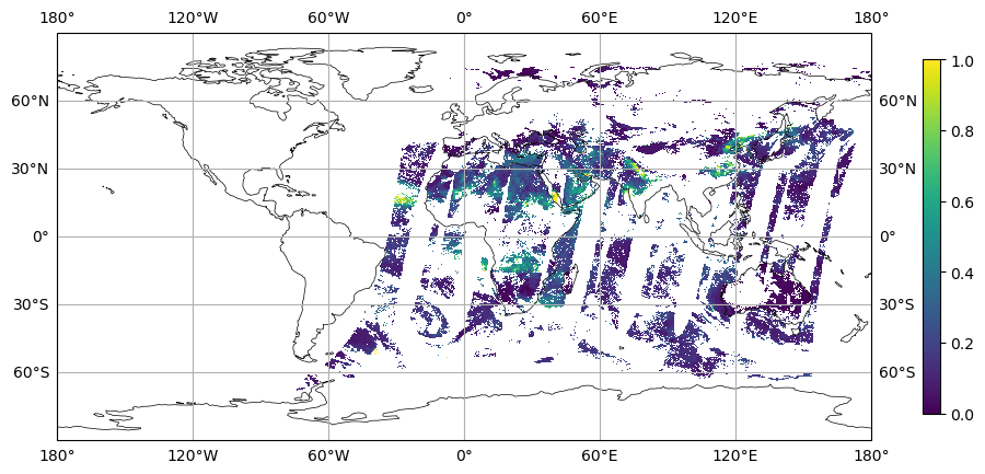
#-- 1. Plot the remapped data
variable = ds_out[var_name].mean('time')
fig, ax = plt.subplots(figsize=(12,6),
subplot_kw=dict(projection=ccrs.PlateCarree()))
ax.set_global()
ax.coastlines(lw=0.5)
ax.gridlines(draw_labels=True)
plot = ax.pcolormesh(x, y, variable, cmap='viridis', vmin=vmin , vmax=vmax)
cbar = plt.colorbar(plot, shrink=0.7)
plt.savefig(f'plot_MODIS_N256_new_ri{ri}_epsilon{epsilon}_1.png',
bbox_inches='tight',
facecolor='white')
plt.show()
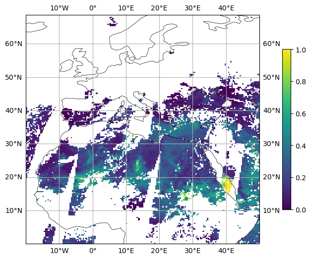
#-- 2. Zoom in
fig, ax = plt.subplots(figsize=(12,6),
subplot_kw=dict(projection=ccrs.PlateCarree()))
ax.set_extent([-20., 50., 0., 65.])
ax.coastlines(lw=0.5)
ax.gridlines(draw_labels=True)
plot = ax.pcolormesh(x, y, variable, cmap='viridis', vmin=vmin, vmax=vmax)
cbar = plt.colorbar(plot, shrink=0.7)
plt.savefig(f'plot_MODIS_N256_new_ri{ri}_epsilon{epsilon}_2.png',
bbox_inches='tight',
facecolor='white')
plt.show()
Plot result#