Python: Mollweide projection problem

Description

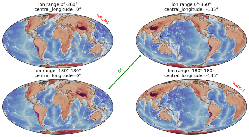
The use of the Mollweide projection can in some cases lead to an unsightly ‘stripe effect’ at the poles, as the data is not mapped correctly onto the map.

If the data is in the longitude value range -180°-180° then everything is OK. If the data is available in an longitude value range of 0°-360°, this can lead to a striped effect at the poles. Unfortunately, the same effect also occurs if the data is available in the correct longitude value range, but the map center point (central_longitude) is changed from 0° for example to -135°.

Software requirements

• Python 3

• matplotlib

• cartopy

• python-cdo

Example script

Mollweide_projection_problem.py

#!/usr/bin/env python
# coding: utf-8
#
# Mollweide - central_longitude
# 
# 2025 copyright DKRZ licensed under CC BY-NC-ND 4.0 
#                     (https://creativecommons.org/licenses/by-nc-nd/4.0/deed.en)
# 
# The use of the Mollweide projection can in some cases lead to an unsightly '
# stripe effect' at the poles, as the data is not mapped correctly onto the map.
# 
# If the data is in the longitude value range -180°-180° then everything is OK. 
# If the data is available in an longitude value range of 0°-360°, this can lead 
# to a striped effect at the poles.  Unfortunately, the same effect also occurs 
# if the data is available in the correct longitude value range, but the map 
# center point (central_longitude) is changed from 0° for example to -135°.
# 
#
# central_longitude 	dataset longitude range 	plot result
#		0.					-180° - 180°				ok
#		0. 					   0° - 360° 			wrong
#	 -135. 					-180° - 180° 			wrong
#	 -135. 				       0° - 360° 			ok

#-- import packages
import matplotlib.pyplot as plt
import matplotlib.lines as mlines
import cartopy.crs as ccrs
import cartopy.feature as cfeature
from cdo import Cdo
cdo = Cdo()

#-- Example data
# 
# We generate the example data as Xarray dataset from the topography dataset from 
# the Climet Data Operators (CDO). One dataset with the longitude value range 
# 0°-360° (ds0) and another dataset with the longitude value range -180°-180° (ds1).
ds0 = cdo.sellonlatbox('0.,360.,-90.,90.', input='-topo,global_1', returnXDataset=True)
ds1 = cdo.topo('global_1', returnXDataset=True)

# Print the longitude ranges of the two datasets.
print(f'longitude range:  {ds0.lon.min().values} - {ds0.lon.max().values}')
print(f'longitude range:  {ds1.lon.min().values} - {ds1.lon.max().values}')

#-- Define Mollweide projection with different central_longitude
# 
# To demonstrate the 'stripe effect' we use the default central_longitude=0° 
# setting and as a second setting central_longitude=-135°.
central_longitude0 = 0.
central_longitude1 = -135.  

proj0 = ccrs.Mollweide(central_longitude=central_longitude0)
proj1 = ccrs.Mollweide(central_longitude=central_longitude1)

#-- Global plots
# 
# Create the Mollweide projection plots for the two datasets using the two 
# different central_longitude values.

#-- color map
cmap = 'twilight_shifted'

fig = plt.figure(figsize=(12,6))
gs = fig.add_gridspec(2, 2, height_ratios=[1,1])

#-- 1. plot
ax1 = fig.add_subplot(gs[0,0], projection = proj0)
ax1.set_title(f'lon range 0°-360°\ncentral_longitude=0°')
ax1.coastlines(lw=0.3, zorder=2)
plot1 = ax1.pcolormesh(ds0.lon, ds0.lat, ds0.topo, cmap=cmap, 
                       transform=ccrs.PlateCarree())

#-- 2. plot
ax2 = fig.add_subplot(gs[0,1], projection = proj1)
ax2.set_title(f'lon range 0°-360°\ncentral_longitude=-135°')
ax2.coastlines(lw=0.3, zorder=2)
plot2 = ax2.pcolormesh(ds0.lon, ds0.lat, ds0.topo, cmap=cmap, 
                       transform=ccrs.PlateCarree())

#-- 3. plot
ax3 = fig.add_subplot(gs[1,0], projection = proj0)
ax3.set_title(f'lon range -180°-180°\ncentral_longitude=0°')
ax3.coastlines(lw=0.3, zorder=2)
plot3 = ax3.pcolormesh(ds1.lon, ds1.lat, ds1.topo, cmap=cmap, 
                       transform=ccrs.PlateCarree())

#-- 4. plot
ax4 = fig.add_subplot(gs[1,1], projection = proj1)
ax4.set_title(f'lon range -180°-180°\ncentral_longitude=-135°')
ax4.coastlines(lw=0.3, zorder=2)
plot4 = ax4.pcolormesh(ds1.lon, ds1.lat, ds1.topo, cmap=cmap, 
                       transform=ccrs.PlateCarree())

#-- add an arrow between the correct subplots
arrowprops = dict(arrowstyle="<->", linewidth=2, color='green')
arrow1_2 = plt.annotate('', xy=(0.05, 0.25), xycoords=ax2.transAxes, 
                        xytext=(0.95, 0.8), textcoords=ax3.transAxes, 
                        arrowprops=arrowprops)
#-- add text
plt.text(0.49, 0.5,  'OK',    color='green', rotation=45,  transform=fig.transFigure)
plt.text(0.42, 0.81, 'WRONG', color='red',   rotation=325, transform=fig.transFigure)
plt.text(0.85, 0.38, 'WRONG', color='red',   rotation=325, transform=fig.transFigure)

plt.savefig('plot_mollweide_global.png', bbox_inches='tight', dpi=150);

#-- Closer look at the poles
# 
# Let's have a closer look at the pole regions for each of the examples from above.
fig = plt.figure(figsize=(12,4.8))
gs = fig.add_gridspec(4, 2)

#---------------
#-- wrong plots
#---------------
#-- 5. plot
ax5 = fig.add_subplot(gs[0,0], projection = proj0)
ax5.set_title(f'$\\bf WRONG: $\nlon range 0°-360°\ncentral_longitude=0', fontsize=10)
ax5.set_extent([0,360,75,90], crs=ccrs.PlateCarree())
ax5.coastlines(lw=0.3, zorder=2)
plot5 = ax5.pcolormesh(ds0.lon, ds0.lat, ds0.topo, cmap=cmap, transform=ccrs.PlateCarree())

#-- 6. plot
ax6 = fig.add_subplot(gs[0,1], projection = proj0)
ax6.set_title(f'$\\bf WRONG: $\nlon range 0°-360°\ncentral_longitude=0', fontsize=10)
ax6.set_extent([0,360,-90,-75], crs=ccrs.PlateCarree())
ax6.coastlines(lw=0.3, zorder=2);
plot6 = ax6.pcolormesh(ds0.lon, ds0.lat, ds0.topo, cmap=cmap, transform=ccrs.PlateCarree())

#-- 7. plot
ax7 = fig.add_subplot(gs[1,0], projection = proj1)
ax7.set_title(f'$\\bf WRONG: $\nlon range -180°-180°\ncentral_longitude=-135.', fontsize=10)
ax7.set_extent([0,360,75,90], crs=ccrs.PlateCarree())
ax7.coastlines(lw=0.3, zorder=2)
plot7 = ax7.pcolormesh(ds1.lon, ds1.lat, ds1.topo, cmap=cmap, transform=ccrs.PlateCarree())

#-- 8. plot
ax8 = fig.add_subplot(gs[1,1], projection = proj1)
ax8.set_title(f'$\\bf WRONG: $\nlon range -180°-180°\ncentral_longitude=-135.', fontsize=10)
ax8.set_extent([0,360,-90,-75], crs=ccrs.PlateCarree())
ax8.coastlines(lw=0.3, zorder=2);
plot8 = ax8.pcolormesh(ds1.lon, ds1.lat, ds1.topo, cmap=cmap, transform=ccrs.PlateCarree())

#-- draw a horizontal line
fig.add_artist(mlines.Line2D([0.12, 0.9], [0.54, 0.54], color='gray', ls='--', lw=2))

#-----------------
#-- correct plots
#-----------------
#-- 9. plot
ax9 = fig.add_subplot(gs[2,0], projection = proj0)
ax9.set_title(f'$\\bf OK: $\nlon range -180°-180°\ncentral_longitude=0', fontsize=10)
ax9.set_extent([0,360,75,90], crs=ccrs.PlateCarree())
ax9.coastlines(lw=0.3, zorder=2)
plot9 = ax9.pcolormesh(ds1.lon, ds1.lat, ds1.topo, cmap=cmap, transform=ccrs.PlateCarree())

#-- 10. plot
ax10 = fig.add_subplot(gs[2,1], projection=proj0)
ax10.set_title(f'$\\bf OK: $\nlon range -180°-180°\ncentral_longitude=0', fontsize=10)
ax10.set_extent([0,360,-90,-75], crs=ccrs.PlateCarree())
ax10.coastlines(lw=0.3, zorder=2)
plot10 = ax10.pcolormesh(ds1.lon, ds1.lat, ds1.topo, cmap=cmap, transform=ccrs.PlateCarree())

#-- 11.plot
ax11 = fig.add_subplot(gs[3,0], projection = proj1)
ax11.set_title(f'$\\bf OK: $\nlon range 0°-360°\ncentral_longitude=-135', fontsize=10)
ax11.set_extent([0,360,75,90], crs=ccrs.PlateCarree())
ax11.coastlines(lw=0.3, zorder=2)
plot11 = ax11.pcolormesh(ds0.lon, ds0.lat, ds0.topo, cmap=cmap, transform=ccrs.PlateCarree())

#-- 12. plot
ax12 = fig.add_subplot(gs[3,1], projection=proj1)
ax12.set_title(f'$\\bf OK: $\nlon range 0°-360°\ncentral_longitude=-135', fontsize=10)
ax12.set_extent([0,360,-90,-75], crs=ccrs.PlateCarree())
ax12.coastlines(lw=0.3, zorder=2)
plot12 = ax12.pcolormesh(ds0.lon, ds0.lat, ds0.topo, cmap=cmap, transform=ccrs.PlateCarree())

#-- add annotation on the upper left side of the figure
plt.text(0.5, 0.95, 'Mollweide', fontsize=14, weight='bold', ha='center', transform=fig.transFigure)
plt.text(0.5, 0.92, 'central_longitude / lon range', fontsize=10, ha='center', transform=fig.transFigure)

plt.savefig('plot_mollweide_poles.png', bbox_inches='tight', dpi=150);

Plot result