Python shapefile basics#
Description
The following example gives a brief overview of how to easily read in a shapefile using the GeoPandas software package and use it for visualization.
The used shapefile from data.dtu.dk contains the border lines of the European countries.
Learning steps:
read the data into a GeoPandas DataFrame
- have a closer look at the content
country (DataFrame row), abbreviation and name (DataFrame columns)
country area (DataFrame geometry, polygons)
country borderline (DataFrame geometry, polylines)
extract the data for a single country
extract the data for multiple countries
plot geometries
- combine GeoPandas plotting routine with Matplotlib and Cartopy
draw country borderline over data (overlay) on a map
Software requirements
Python 3
geopandas
matplotlib
cartopy
xarray
Notebook shapefile_basics.ipynb
Example script#
shapefile_basics.py
#!/usr/bin/env python
# coding: utf-8
'''
DKRZ Tutorial
Shapefiles
The following example gives a brief overview of how to easily read in a
shapefile using the GeoPandas software package and use it for visualization.
The used shapefile from data.dtu.dk contains the border lines of the
European countries.
Learning steps
- read the data into a GeoPandas DataFrame
- have a closer look at the content
- country (DataFrame row), abbreviation and name (DataFrame columns)
- country area (DataFrame geometry, polygons)
- country borderline (DataFrame geometry, polylines)
- extract the data for a single country
- extract the data for multiple countries
- plot geometries
- combine GeoPandas plotting routine with Matplotlib and Cartopy
- draw country borderline on data (overlay)
GeoPandas
URL: https://geopandas.org/en/stable/
Shapefile description
From the ESRI Shapefile Technical Description
https://www.esri.com/content/dam/esrisites/sitecore-archive/Files/Pdfs/library/whitepapers/pdfs/shapefile.pdf
A shapefile stores nontopological geometry and attribute information for
the spatial features in a data set. The geometry for a feature is stored
as a shape comprising a set of vector coordinates.
Because shapefiles do not have the processing overhead of a topological
data structure, they have advantages over other data sources such as faster
drawing speed and edit ability. Shapefiles handle single features that
overlap or that are noncontiguous. They also typically require less disk
space and are easier to read and write.
Shapefiles can support point, line, and area features. Area features are
represented as closed loop, double-digitized polygons. Attributes are held
in a dBASE® format file.
Each attribute record has a one-to-one relationship with the associated
shape record.
Download shapefile
Shapefile download page:
https://data.dtu.dk/articles/dataset/Shapefile_of_European_countries/23686383
Used shapefile data set:
https://data.dtu.dk/ndownloader/articles/23686383/versions/1
Sevdari, Kristian; Marmullaku, Drin (2023). Shapefile of European countries.
Technical University of Denmark. Dataset. https://doi.org/10.11583/DTU.23686383.v1
-------------------------------------------------------------------------------
2024 copyright DKRZ licensed under CC BY-NC-SA 4.0
(https://creativecommons.org/licenses/by-nc-sa/4.0/deed.en)
-------------------------------------------------------------------------------
'''
from datetime import datetime
import geopandas as gpd
import matplotlib.pyplot as plt
from matplotlib.lines import Line2D
import cartopy.crs as ccrs
import cartopy.feature as cfeature
def main():
plt.switch_backend('agg')
# Load the shapefile
#
# 1. Download the shapefile from https://data.dtu.dk/ndownloader/articles/23686383/versions/1
#
# 2. Load the shapefile with GeoPandas `read_file()` function.
shapefile_path = '../../data/Europe_merged.shp'
gdf = gpd.read_file(shapefile_path)
# Shapefile content
#
# Print the first 5 lines of the shapefile content using the `.head()` method.
print(gdf.head())
# Shape, rows, and columns
#
# The readonly property `shape` gives us the (nrows, ncols) size of the
# DataFrame.
print(gdf.shape)
# Number of rows
nrows = gdf.shape[0]
print(nrows)
# same as above
nrows = len(gdf.index)
print(nrows)
# Number of columns
ncols = gdf.shape[1]
print(ncols)
# same as above
ncols = len(gdf.columns)
print(ncols)
# Each row in the GeoPandas DataFrame contains the data of one country.
#
# Select a row by index
print(gdf.iloc[10])
print('----------------------')
print(gdf.iloc[10].GID_0)
print(gdf.iloc[10].COUNTRY)
print(gdf.iloc[10].name)
# To print the column names use the `columns` method.
print(gdf.columns.values)
# Select a row (= country) by its name, therefore, we use the column COUNTRY
# for the condition.
print(gdf.loc[gdf['COUNTRY'] == 'Germany'])
# Bounds
#
# Print the bounds of the first 5 countries.
print(gdf.bounds.head())
# Print bounds range of the shapefile content.
print(f'minx: {min(gdf.bounds.minx):8.3f} maxx: {max(gdf.bounds.maxx):8.3f}')
print(f'miny: {min(gdf.bounds.miny):8.3f} maxy: {max(gdf.bounds.maxy):8.3f}')
# Plot shapefile content
#
# The GeoPandas package provides an interface to Matplotlib for drawing.
# Therefore, we use the GeoPandas function `.plot()` to plot the content of
# the GeoPandas data frame. See also https://geopandas.org/en/stable/docs/user_guide/mapping.html.
gdf.plot()
plt.savefig('plot_shp_1.png', bbox_inches='tight', facecolor='white')
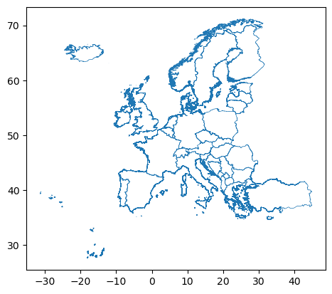
# The plot above shows the drawings of the multi-polygons of the countries
# (default). If you want to draw only the outlines, the border lines of the
# countries, you can use the `.boundary` method with the `.plot()` method.
gdf.boundary.plot(linewidth=0.5)
plt.savefig('plot_shp_2.png', bbox_inches='tight', facecolor='white')
# Draw each country using the columns 'GID_0' or 'COUNTRY'. To add a legend
# to the plot the parameter column has to be given to the plot call. GID_0 for
# the country abbreviation or COUNTRY for the standard name.
legend_kw = dict(loc='center left', bbox_to_anchor=(1,0.5), fontsize=6, ncols=3)
gdf.plot(column='COUNTRY', cmap='gist_rainbow', figsize=(12, 5),
legend=True, legend_kwds=legend_kw) # standard names
#gdf.plot(column='GID_0', cmap='gist_rainbow', figsize=(12, 5),
# legend=True, legend_kwds=legend_kw) # abbreviations
plt.savefig('plot_shp_3.png', bbox_inches='tight', facecolor='white')
# Extract countries
#
# We can extract a single country or a set of countries as shown above with
# the `loc` and `iloc` methods, but there is a third method called `where`
# that can do it as well.
#
# Using `where` method
gdf.where(gdf['COUNTRY'] == 'Germany' ).plot()
plt.savefig('plot_shp_4.png', bbox_inches='tight', facecolor='white')
# Here, we use the `loc` method of the GeoPandas DataFrame to extract the
# geometries of Germany, and assign it to a variable.
D = gdf.loc[gdf['COUNTRY'] == 'Germany']
print(D)
# Extract multiple countries using `query()` method
#
# The `query()` method allows us to pass a list of country names for the
# selection.
country_list = ['Germany', 'France']
countries = gdf.query('COUNTRY in @country_list')
print(countries)
countries.plot()
plt.savefig('plot_shp_5.png', bbox_inches='tight', facecolor='white')
# Print the index
cindex = countries.index.values
print(cindex)
# Print the multi-polygon geometries
print(countries.geometry)
# Get the bounds of the two countries, the minimum and maximum of the
# multipolygon coordinate data.
print(countries.bounds)
# Print the polyline data of the multi-polygon.
print(countries.boundary)
countries.boundary.plot(lw=0.5)
plt.savefig('plot_shp_6.png', bbox_inches='tight', facecolor='white')
# Shapefile projection
#
# In most cases the geometries of a shapefile based on a projection. We can
# get the stored projection with the `crs` property.
print(countries.crs)
# Plotting with Matplotlib
#
# Sometimes you'll want to have more controll on the plot creation and that
# is why we here combine the plot functionalities of GeoPandas, Matplotlib,
# and Cartopy.
#
# First, we select each geometry for the two countries Germany and France.
# We do this in order to have better control over the individual plots of the
# countries, e.g. the choice of colors, hatching or the respective labels for
# the legend.
D = gdf.loc[gdf['COUNTRY'] == 'Germany']
F = gdf.loc[gdf['COUNTRY'] == 'France']
# In the next step, we
#
# - draw the two countries on a map,
# - zoom into the map,
# - add a legend to the right side of the plot
proj = ccrs.PlateCarree()
fig, ax = plt.subplots(figsize=(6,4), subplot_kw={'projection': proj},
layout='tight')
ax.set_extent([-6., 16., 40., 57.])
ax.gridlines(draw_labels=True, color='gray', alpha=0.8, linestyle='--')
style_kwds = dict(color='gold', edgecolor='red', hatch='///', linewidth=0.6,)
D.plot(ax=ax, **style_kwds, transform=ccrs.PlateCarree())
style_kwds = dict(color='blue', edgecolor='red', linewidth=0.6,)
F.plot(ax=ax, **style_kwds, transform=ccrs.PlateCarree())
legend_labels = ['Germany (D)', 'France (F)']
legend_item1 = Line2D([], [], linestyle='none', color='gold', marker='o', markerfacecolor="gold")
legend_item2 = Line2D([], [], linestyle='none', color='blue', marker='o', markerfacecolor="blue")
legend_marker = (legend_item1, legend_item2)
plt.legend(handles=legend_marker, labels=legend_labels, loc=(1.1, 0.92), fontsize=8)
ax.add_feature(cfeature.LAND.with_scale('50m'), color='whitesmoke', zorder=0)
ax.add_feature(cfeature.OCEAN.with_scale('50m'), color='lightgray', zorder=0);
plt.savefig('plot_shp_7.png', bbox_inches='tight', facecolor='white')
# Re-project to Orthographic projection
#
# To plot the pre-projected shapefile content correctly, we have to re-project
# it to the target projection, here Orthographic. Therefore, we can use the
# `to_crs()` method of the GeoPandas GeoDataFrame with the PROJ string from
# Cartopy's CRS of the target projection.
#
# Target projection
proj = ccrs.Orthographic(central_longitude=0., central_latitude=52.)
# Generate PROJ string from Cartopy CRS
proj_string = proj.proj4_init
print(proj_string)
# Re-project geometries of the GeoPandas GeoDataFrames D and F.
D_ortho = D.to_crs(proj_string)
F_ortho = F.to_crs(proj_string)
# **Note:**
# Due to the fact that we re-project the shapefile geometries for the selected
# countries, we do not need to use the transform parameter in the plot call.
#
# In the next step, we
#
# - draw the two countries on a map with Orthographic projection,
# - zoom into the map,
# - choose different colors and hatching,
# - add a legend to the right side of the plot
start_time = datetime.now()
fig, ax = plt.subplots(figsize=(6,4), subplot_kw={'projection': proj},
layout='tight')
ax.set_extent([-30., 40., 20., 75.])
ax.gridlines(draw_labels=True, color='gray', alpha=0.8, linestyle='--')
ax.coastlines(resolution='50m', linewidth=0.6, edgecolor='black')
style_kw = dict(color='gold', edgecolor='red', hatch='///', linewidth=0.6,)
D_ortho.plot(ax=ax, **style_kw)
style_kw = dict(color='blue', edgecolor='red', linewidth=0.6,)
F_ortho.plot(ax=ax, **style_kw)
legend_labels = ['Germany (D)', 'France (F)']
legend_item1 = Line2D([], [], linestyle='none', color='gold', marker='o', markerfacecolor='gold')
legend_item2 = Line2D([], [], linestyle='none', color='blue', marker='o', markerfacecolor='blue')
legend_marker = (legend_item1, legend_item2)
plt.legend(handles=legend_marker, labels=legend_labels, loc=(1.1, 0.92), fontsize=8)
print(f'run time: {datetime.now() - start_time}\n')
plt.savefig('plot_shp_8.png', bbox_inches='tight', facecolor='white')
# Make it faster with Cartopy's `ax.add_geometries()`
#
# A faster way to generate the plot of the map with the shapefile geometries
# is to use Cartopy's `ax.add_geometries()` method instead of geoDataFrame.plot().
start_time = datetime.now()
fig, ax = plt.subplots(figsize=(6,4), subplot_kw={'projection': proj},
layout='tight')
ax.set_extent([-30., 40., 20., 75.])
ax.gridlines(draw_labels=True, color='gray', alpha=0.8, linestyle='--')
ax.coastlines(resolution='50m', linewidth=0.6, edgecolor='black')
style_kw = dict(facecolor='gold', edgecolor='red', hatch='///', linewidth=0.6,)
ax.add_geometries(D_ortho["geometry"], crs=proj, **style_kw)
style_kw = dict(facecolor='blue', edgecolor='red', linewidth=0.6,)
ax.add_geometries(F_ortho["geometry"], crs=proj, **style_kw,)
legend_labels = ['Germany (D)', 'France (F)']
legend_item1 = Line2D([], [], linestyle='none', color='gold', marker='o', markerfacecolor='gold')
legend_item2 = Line2D([], [], linestyle='none', color='blue', marker='o', markerfacecolor='blue')
legend_marker = (legend_item1, legend_item2)
plt.legend(handles=legend_marker, labels=legend_labels, loc=(1.1, 0.92), fontsize=8)
print(f'run time: {datetime.now() - start_time}\n')
plt.savefig('plot_shp_9.png', bbox_inches='tight', facecolor='white')
# Overlay, draw borderlines over data
#
# For the sake of simplicity, we use an example data set provided by the
# **Xarray** package. See also https://docs.xarray.dev/en/stable/generated/xarray.tutorial.open_dataset.html
#
# The data set we use here contains the variable **rasm** which is the output
# of the Regional Arctic System Model (RASM).
#
# **Note:**
# The variable **Tair** has the coordinates (time,y,x) where x and y are the
# logical coordinates that point to the physical coordinate variables xc and yc.
# The physical coordinates xc,yc are 2-dimensional arrays.
import xarray as xr
ds = xr.tutorial.open_dataset('rasm')
print(ds)
# Select the first time step
var = ds.Tair.isel(time=0)
# Let's have a quick look at the data. Using the plot() method without further
# parameter settings, the plot routine will use the logical coordinates.
var.plot()
plt.savefig('plot_shp_10.png', bbox_inches='tight', facecolor='white')
# Now, we can use the already known plotting content from above and add the
# data variable using the physical coordinates.
#
# You can use Xarray's or Matplotlib's plot methods. Under the hood, Xarray
# uses the plot functionality of Matplotlib.
#
# In the following we only need the plot commands from above plus a plot
# command for the variable Tair. As there are two ways of plotting the data,
# we create two plots next to each other so that we can compare them more easily.
start_time = datetime.now()
fig, (ax1,ax2) = plt.subplots(nrows=1, ncols=2, figsize=(8,8),
subplot_kw={'projection': proj},
layout='tight')
#-- use Xarray's plot method (uses Matplotlib under the hood)
ax1.set_extent([-30., 40., 20., 75.])
ax1.gridlines(draw_labels=True, color='gray', alpha=0.8, linestyle='--')
ax1.coastlines(resolution='50m', linewidth=0.6, color='blue')
cn1 = var.plot.pcolormesh(ax=ax1, x='xc', y='yc',
cmap='RdBu_r',
add_colorbar=False,
transform=ccrs.PlateCarree())
ax1.set_title('')
#-- use Matplotlib's plot method
ax2.set_extent([-30., 40., 20., 75.])
ax2.gridlines(draw_labels=True, color='gray', alpha=0.8, linestyle='--')
ax2.coastlines(resolution='50m', linewidth=0.6, color='blue')
cn2 = ax2.pcolormesh(ds.xc, ds.yc, var,
cmap='RdBu_r',
transform=ccrs.PlateCarree())
#-- add geometries to both plots
style_kw = dict(facecolor='None', edgecolor='black', linewidth=0.5)
ax1.add_geometries(D_ortho["geometry"], crs=proj, **style_kw)
ax1.add_geometries(F_ortho["geometry"], crs=proj, **style_kw,)
ax2.add_geometries(D_ortho["geometry"], crs=proj, **style_kw)
ax2.add_geometries(F_ortho["geometry"], crs=proj, **style_kw,)
print(f'run time: {datetime.now() - start_time}\n')
plt.savefig('plot_shp_11.png', bbox_inches='tight', facecolor='white')
# **Conclusion:** with GeoPandas, shapefiles can be used in a very simple way.
if __name__ == '__main__':
main()
Plot result#