Python use a shapefile for masking data#
Description
In this tutorial we will use as sample data CDO’s topography data set. In the first example we extract and draw the data for a single German state, in the second example for Germany, and in the third example we take a shapefile containing the features of almost all countries to draw the data for one selected country.
Learning steps:
read the data into a GeoPandas DataFrame
have a closer look at the content
generate topography dataset
extract the geometries for a single state or country
plot geometries
generate the mask array to be used for drawing data only in the area of the selected state or country
Software requirements
Python 3
geopandas
regionmask
matplotlib
cartopy
xarray
python-cdo
python shapefile_to_mask_data.py
Notebook shapefile_to_mask_data.ipynb
Example script#
shapefile_to_mask_data.py
#!/usr/bin/env python
# coding: utf-8
'''
DKRZ Tutorial
Masking data using shapefiles
In the field of data analysis and visualization, in some cases you want to
use or display only the data of a certain geographical region. Selecting data
of a certain region can be done, among other things, with the help of a
shapefile for this region. Shapefiles contain georeferenced points, lines,
and/or area features and can be downloaded from different sites.
In this tutorial we will use as sample data CDO's topography data set. In
the first example we extract and draw the data for a single German state,
in the second example for Germany, and in the third example we take a
shapefile containing the features of almost all countries to draw the data
for one selected country.
Content
- Function: shp_mask_var()
- Read a shapefile
- Generate sample data - topo
a. Plotting with ax.add_feature()
b. Plotting with ax.add_geometries()
- Example 1: Draw sample data of selected German state
- Example 2: Draw the data of variable topo of the area of Germany
- Example 3: Using the world countries.shp
Shapefile description
From the _ESRI Shapefile Technical Description_
https://www.esri.com/content/dam/esrisites/sitecore-archive/Files/Pdfs/library/whitepapers/pdfs/shapefile.pdf
A shapefile stores nontopological geometry and attribute information for
the spatial features in a data set. The geometry for a feature is stored
as a shape comprising a set of vector coordinates.
Because shapefiles do not have the processing overhead of a topological
data structure,they have advantages over other data sources such as faster
drawing speed and edit ability. Shapefiles handle single features that
overlap or that are noncontiguous. They also typically require less disk
space and are easier to read and write.
Shapefiles can support point, line, and area features. Area features are
represented as closed loop, double-digitized polygons. Attributes are
held in a dBASE® format file. Each attribute record has a one-to-one
relationship with the associated shape record.
Shapefiles used
- gadm36_DEU_shp/gadm36_DEU_0.shp
- gadm36_DEU_shp/gadm36_DEU_1.shp
- countries_shp/countries.shp
Learning content
- Read shapefile content
- Extract polygon data of the choosen shapefile content
- Generate a mask array and use it to mask variable data
- Plot the masked data
Shapefile download sites: just google 'shapefile download'
-------------------------------------------------------------------------------
2024 copyright DKRZ licensed under CC BY-NC-SA 4.0
(https://creativecommons.org/licenses/by-nc-sa/4.0/deed.en)
-------------------------------------------------------------------------------
'''
import os
from datetime import datetime
import xarray as xr
import numpy as np
import geopandas as gpd
import regionmask
import matplotlib.pyplot as plt
import cartopy.io.shapereader as shpreader
import cartopy.feature as cfeature
import cartopy.crs as ccrs
from cdo import Cdo
cdo = Cdo()
# Function: shp_mask_var()
#
# This function reads the content of a shapefile, extracts the shapefile
# variable geometry data with the use of the given 'name' parameter, and
# generates the mask array. It uses GeoPandas's read_file() and regionmask's
# Regions() methods.
def shp_mask_var(ds, varname, shpfile, name, shpvar, lat_name='lat', lon_name='lon'):
'''
Reads the shapefile content and extract the chosen name to be used to extract
the variable data.
Keywords:
ds Dataset containing the variable and the dimensions time, lat, lon
varname data variable name
shpfile shapefile name
shpvar shapefile variable to extract, e.g. NAME_1
lat_name latitude coordinate name
lon_name longitude coordinate name
returns mask array
Requirements:
geopandas
regionmask
'''
#-- read the shapefile
content = gpd.read_file(shpfile)
#-- get the index of the given name in the shapefile
index = content[content[shpvar] == name].index.values
#-- number of rows in GeoDataFrame
nindex = content.index.size
#-- create a Region object for the shapefile content
content_mask = regionmask.Regions(name = list(content[shpvar])[0],
numbers = list(range(0,nindex)),
names = list(content[shpvar]),
abbrevs = list(content[shpvar]),
outlines = list(content.geometry.values[i] for i in range(0,nindex)))
#-- create the mask array with same grid size as the data variable
mask = content_mask.mask(ds, lat_name=lat_name, lon_name=lon_name)
mask = mask.where(mask == index)
#-- return the dataset that contains the variable data with the generated
# mask array
return ds[varname].where(mask == index)
#-- main
def main():
plt.switch_backend('agg')
# Read a shapefile
#
# The shapefile gadm36_DEU_1.shp contains the border polygons of the 16
# federal states of Germany.
shp_file = '../../data/gadm36_DEU_1.shp'
# Read the shapefile content using GeoPandas's read_file() method.
gdf = gpd.read_file(shp_file)
#-- print the first 3 rows
print(gdf.head(3))
# Generate sample data - topo
#
# Here, we use the topo operator of CDO to generate a global 0.1°x0.1°
# topography sample data set.
cdo.remapnn('global_0.1', input='-topo', options='-O -f nc', output='topo.nc')
var_name = 'topo'
ds = xr.open_dataset('topo.nc')
#print(ds.topo)
#-- Example 1: Draw sample data of selected German state
#
# The first example shows how to extract the geometry data of a single state
# from the shapefile and use it to generate the mask array.
name = 'Niedersachsen'
#name = 'Schleswig-Holstein'
#name = 'Bayern'
# The geometry data for each German state is stored in the shapefile variable
# NAME_1 in the gadm36_DEU_1.shp file.
shp_var = 'NAME_1'
#-- a. Plotting with ax.add_feature()
#
# Get the shapefile polygon of the choosen German state.
reader = shpreader.Reader(shp_file)
country = [polygon for polygon in reader.records() if polygon.attributes[shp_var] == name][0]
#print(country.geometry)
# Use the function shp_mask_var to generate the masked data.
masked_data = shp_mask_var(ds, var_name, shp_file, name, shp_var)
#print(masked_data)
# Create the plot and zoom into the map to display the area of Germany.
# Here, we use the ax.add_feature() method to add the geometries for drawing
# the German state border line at the end.
start_time = datetime.now()
projection = ccrs.Mercator()
fig, ax = plt.subplots(figsize=(4,4), subplot_kw=dict(projection = projection))
ax.set_extent([5., 16., 47., 55.5])
ax.add_feature(cfeature.BORDERS)
ax.add_feature(cfeature.OCEAN)
ax.add_feature(cfeature.COASTLINE)
plot = ax.pcolormesh(ds.lon.values,
ds.lat.values,
masked_data,
cmap='gist_earth',
transform=ccrs.PlateCarree())
shape_feature = cfeature.ShapelyFeature([country.geometry],
ccrs.PlateCarree(),
facecolor='none',
edgecolor='black',
linewidth=1)
ax.add_feature(shape_feature)
plt.savefig('plot_shp_mask_1.png', bbox_inches='tight', facecolor='white')
print(f'run time: {datetime.now() - start_time}\n')
#-- b. Plotting with ax.add_geometries()
#
# In addition to the ax.add_feature method, the ax.add_geometries method
# can also be used to add the geometries.
#
# country1 = gpd.read_file(shp_file).loc[gdf[shp_var] == name]
#
# fig, ax = plt.subplots(figsize=(4,4), subplot_kw=dict(projection = ccrs.Mercator()))
#
# ax.set_extent([5., 16., 47., 55.5])
# ax.add_feature(cfeature.BORDERS)
# ax.add_feature(cfeature.OCEAN)
# ax.add_feature(cfeature.COASTLINE)
#
# plot = ax.pcolormesh(ds.lon.values,
# ds.lat.values,
# masked_data,
# cmap='gist_earth',
# transform=ccrs.PlateCarree())
#
# style_kw = dict(facecolor='none', edgecolor='black', linewidth=1)
# shape_feature = ax.add_geometries(country1.geometry,
# crs=ccrs.PlateCarree(),
# **style_kw,)
#
# plt.savefig('plot_shp_mask_1b.png', bbox_inches='tight', facecolor='white')
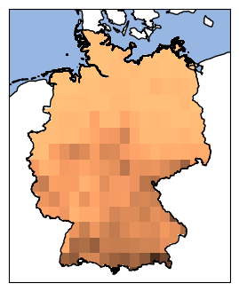
#-- Example 2: Draw the variable in the area of Germany
#
# In the next example we use another shapefile gadm36_DEU_0.shp (not to be
# confused with gadm36_DEU_1.shp) that contains the border polygons of Germany.
#
# The code is more or less the same as the code from the first example. But
# take care about the changed shapefile name and its variable name NAME_0.
shp_file2 = '../../data/gadm36_DEU_0.shp'
name2 = 'Germany'
shp_var2 = 'NAME_0'
reader2 = shpreader.Reader(shp_file2)
country2 = [polygon for polygon in reader2.records() if polygon.attributes[shp_var2] == name2][0]
# Generate the mask array and assign the result to the variable
masked_data2 = shp_mask_var(ds, var_name, shp_file2, name2, shp_var2)
# Create the plot and zoom into the map to display the area of Germany.
projection = ccrs.Mercator()
fig, ax = plt.subplots(figsize=(4,4), subplot_kw=dict(projection=projection))
ax.set_extent([5., 16., 47., 55.5])
ax.add_feature(cfeature.OCEAN)
ax.add_feature(cfeature.COASTLINE)
plot = ax.pcolormesh(ds.lon.values,
ds.lat.values,
masked_data2,
cmap='copper_r',
transform=ccrs.PlateCarree())
shape_feature = cfeature.ShapelyFeature([country2.geometry],
ccrs.PlateCarree(),
facecolor='none',
edgecolor='black',
linewidth=1)
ax.add_feature(shape_feature);
plt.savefig('plot_shp_mask_2.png', bbox_inches='tight', facecolor='white')
#-- Example 3: Using the world countries.shp
#
# In the following example we have the global topography data set and want to
# plot the data of a country. Therefore, we use another shapefile that contains
# the geometries of the countries of the world.
#
# We use the same code as before but have to modify the shapefile name,
# shapefile variable name and country.
#
# Try to extract the data for the areas of the following countries:
# - Australia
# - United States
# - China
# - Antarctica
shp_file3 = '../../data/countries.shp'
# Have a look at the variables in the shapefile.
gpd.read_file(shp_file3).columns
# The shapefile variable NAME contains the names of the countries.
content = gpd.read_file(shp_file3)
#-- print first 5 country names
for x in content['NAME'][0:5]:
print(x)
# Next, we choose the country that we want to extract and generate the masked data.
# Choose the country that has to be masked
#name3 = 'Australia'
#name3 = 'United States'
#name3 = 'China'
#name3 = 'Antarctica'
name3 = 'Canada'
# Select the shapefile variable that contains the polygons for the countries
shp_var3 = 'NAME'
# read shapefile content
reader3 = shpreader.Reader(shp_file3)
# return the polygon of the selected name
country3 = [polygon for polygon in reader3.records() if polygon.attributes[shp_var3] == name3][0]
# Generate the mask array and assign the result to the variable masked_data
masked_data3 = shp_mask_var(ds, var_name, shp_file3, name3, shp_var3)
# Create the plot.
fig, ax = plt.subplots(figsize=(8,4), subplot_kw=dict(projection=ccrs.PlateCarree()))
ax.set_global()
ax.add_feature(cfeature.OCEAN)
ax.add_feature(cfeature.COASTLINE, linewidth=0.3)
plot = ax.pcolormesh(ds.lon.values,
ds.lat.values,
masked_data3,
vmin=0.,
cmap='copper_r',
transform=ccrs.PlateCarree())
shape_feature3 = cfeature.ShapelyFeature([country3.geometry],
ccrs.PlateCarree(),
facecolor='none',
edgecolor='black',
linewidth=0.4)
ax.add_feature(shape_feature3);
plt.savefig('plot_shp_mask_3.png', bbox_inches='tight', facecolor='white')
#-- Zoom in on the map
fig, ax = plt.subplots(figsize=(10,10),
subplot_kw=dict(projection=ccrs.Orthographic(central_longitude=-92,
central_latitude=62)))
ax.set_extent([-127., -57., 41., 84.], crs=ccrs.PlateCarree())
ax.add_feature(cfeature.OCEAN.with_scale('50m'))
ax.add_feature(cfeature.LAKES.with_scale('50m'), lw=0.3, facecolor='none', edgecolor='black')
#ax.add_feature(cfeature.COASTLINE, linewidth=0.3)
ax.gridlines(color='gray', linestyle='--',)
plot = ax.pcolormesh(ds.lon.values,
ds.lat.values,
masked_data3,
vmin=0.,
cmap='copper_r',
transform=ccrs.PlateCarree())
shape_feature3 = cfeature.ShapelyFeature([country3.geometry],
ccrs.PlateCarree(),
facecolor='none',
edgecolor='black',
linewidth=0.4)
ax.add_feature(shape_feature3);
plt.savefig('plot_shp_mask_4.png', bbox_inches='tight', facecolor='white')
#-- And further zoom in on the west coast
fig, ax = plt.subplots(figsize=(10,10),
subplot_kw=dict(projection=ccrs.Orthographic(central_longitude=-126,
central_latitude=50)))
ax.set_extent([-133., -122., 48., 55.], crs=ccrs.PlateCarree())
ax.add_feature(cfeature.OCEAN.with_scale('50m'))
ax.gridlines(color='gray', linestyle='--',)
plot = ax.pcolormesh(ds.lon.values,
ds.lat.values,
masked_data3,
vmin=0.,
cmap='copper_r',
transform=ccrs.PlateCarree())
shape_feature3 = cfeature.ShapelyFeature([country3.geometry],
ccrs.PlateCarree(),
facecolor='none',
edgecolor='black',
linewidth=0.4)
ax.add_feature(shape_feature3);
plt.savefig('plot_shp_mask_5.png', bbox_inches='tight', facecolor='white')
if __name__ == '__main__':
main()
Plot result#