Python: PyVista/GeoVista - CORDEX EUR-11, rotated curvilinear coordinates

Description

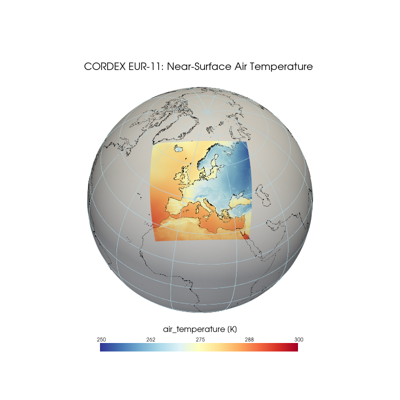
In this example we shows how to plot rotated curvilinear data on a 3d-sphere.

The RCM sample data from CORDEX EUR-11 used here are based on a native one-dimensional grid with rotated coordinates (rlat, rlon). In addition, two-dimensional curvilinear geographic coordinates (lat, lon) are also available.

The data on a curvilinear grid can be transferred to a PyVista mesh using the gv.Transform.from_2d() method, allowing us to plot it directly with geovista.

Content

• Example data

• Plotting - create mesh from 2d-coordinates - create a sphere - plot the mesh on the sphere - add coastlines - add gridlines

Software requirements

• Python 3

• numpy

• xarray

• pyvista

• geovista

Example script

pyvista_CORDEX_EUR11_rotated_curvilinear_grid.py

#!/usr/bin/env python
# coding: utf-8
#
#------------------------------------------------------------------------------
#-- DKRZ example: PyVista/Geovista - CORDEX EUR-11, rotated curvilinear coordinates
#-- 
#-- The RCM sample data from CORDEX EUR-11 used here are based on a native 
#-- one-dimensional grid with rotated coordinates (rlat, rlon). In addition, 
#-- two-dimensional curvilinear geographic coordinates (lat, lon) are also 
#-- available.
#-- 
#-- The data on a curvilinear grid can be transferred to a PyVista mesh using 
#-- the `gv.Transform.from_2d()` method, allowing us to plot it directly with 
#-- geovista.
#-- 
#-- EURO-CORDEX: https://euro-cordex.net/index.php.en <br>
#-- PyVista: https://docs.pyvista.org/ <br>
#-- GeoVista: https://geovista.readthedocs.io/en/stable/index.html <br>
#-- 
#------------------------------------------------------------------------------
#-- 
#-- 2026 copyright DKRZ licensed under CC BY-NC-SA 4.0 
#--                 (https://creativecommons.org/licenses/by-nc-sa/4.0/deed.en)
#-- 
#------------------------------------------------------------------------------
import os
import pyvista as pv
import geovista as gv
import numpy as np
import xarray as xr


#------------------------------------------------------------------------------
#-- CORDEX EUR-11 example data
#------------------------------------------------------------------------------

#-- data file name
file_name = os.environ['HOME'] + '/data/CORDEX/EUR-11/tas_EUR-11_MPI-M-MPI-ESM-LR_rcp45_r1i1p1_CLMcom-CCLM4-8-17_v1_mon_200601-201012.nc'

#-- variable name
var_name = 'tas'

#-- open the file and choose the variable
ds = xr.open_dataset(file_name)
var = ds[var_name]

#-- defining the range of data values to be plotted
var_min, var_max = 250., 300.

#------------------------------------------------------------------------------
#-- Create the mesh
#-- 
#-- "In PyVista, a mesh is any spatially referenced information and usually 
#--  consists of geometrical representations of a surface or volume in 3D space." 
#--  From https://docs.pyvista.org/user-guide/what-is-a-mesh.html
#------------------------------------------------------------------------------

#-- Geovista offers us an easy way to transfer our data from the curvilinear 
#-- grid to a mesh using the `gv.Transform.from_2d()` method. 
mesh = gv.Transform.from_2d(var.lon,
                            var.lat,
                            data=var.isel(time=0),
                            name=f"{var.standard_name} / {var.units}")

#-- remove cells from the mesh with missing values
mesh = mesh.threshold()

#------------------------------------------------------------------------------
#-- Plotting
#-- 
#-- That's all we need to generate a plot. First, we create a sphere onto which 
#-- the data will be projected. Gridlines, coastlines, and a title string are 
#-- also essential, of course. Finally, we change the camera position and add a 
#-- weak light source.
#------------------------------------------------------------------------------

#-- create "geospatial aware plotter" object
plotter = gv.GeoPlotter(window_size=(800,800))

#-- add a title string
title = f'CORDEX EUR-11: {var.long_name}'
plotter.add_text(title, 
                 viewport=True,
                 position=(0.21, 0.82), 
                 font_size=10)

#-- add a sphere
res = 200
radius = 1.
sphere = pv.Sphere(radius=radius, theta_resolution=res, phi_resolution=res)
plotter.add_mesh(sphere, color='gainsboro')

#-- add the mesh
actor = plotter.add_mesh(mesh, 
                         cmap='RdYlBu_r', 
                         opacity=1.,
                         show_scalar_bar=False)
actor.mapper.scalar_range = var_min, var_max

#-- add scalar bar
sbar_args = dict(interactive=False,
                 vertical=False,
                 n_labels=5,
                 title_font_size=16,
                 label_font_size=10,
                 outline=False,
                 width=0.5,
                 height=0.06,
                 position_x= 0.25,
                 position_y= 0.12,
                 fmt='{0:5.0f}')
sbar = plotter.add_scalar_bar(f'{var.standard_name} [{var.units}]', 
                              **sbar_args)
#-- add more space between scalar bar title and the color labels
sbar.GetTitleTextProperty().SetLineOffset(-10.)

#-- add coastlines
plotter.add_coastlines(color='black', line_width=0.1)

#-- add gridlines
plotter.add_graticule(show_labels=False, lon_step=30, lat_step=15)

#-- set camera
plotter.camera.zoom(1.3)
plotter.camera_position = 'yz'
plotter.camera.azimuth = 10     #-- move camera westward
plotter.camera.elevation = 45   #-- move camera northward
plotter.camera.roll -= 5        #-- rotate the camera

#-- light settings
light = pv.Light()
light.set_direction_angle(0, 0)   #-- +x-direction
light.intensity = 0.25            #-- set light intensity to x%
plotter.add_light(light)

#-- display the result and save output to PNG
plotter.show(screenshot='plot_pyvista_rotated_curvilinear_grid.png')

Plot result