Python: PyVista/GeoVista - 3D - wind arrows on a sphere#
Description
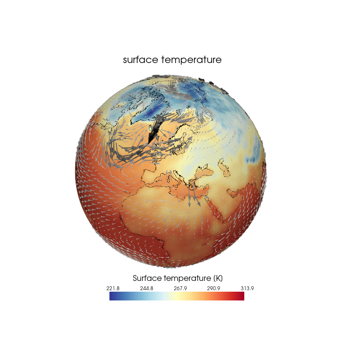
This example demonstrates how to plot the u and v components of the wind on a 3D sphere. To do this, the data must be transformed into the Cartesian coordinate system.
The function generate_vector_mesh() defined here is based on the example ‘Plot data in spherical coordinates’ by PyVista at https://docs.pyvista.org/examples/02-plot/spherical.html
The script generates a total of 4 plots, and only the last one is shown below.
Content
Example data
create mesh from 1d-coordinates
create mesh for the vectors
plot the meshes
add coastlines
Software requirements
Python 3
numpy
xarray
pyvista
geovista
cartopy
Example script#
pyvista_geovista_wind_arrows.py
#!/usr/bin/env python
# coding: utf-8
#------------------------------------------------------------------------------
#-- PyVista / GeoVista: Wind vectors (arrows) on the sphere
#--
#-- This example demonstrates how to plot the u and v components of the wind on
#-- a 3D sphere. To do this, the data must be transformed into the Cartesian
#-- coordinate system.
#--
#-- The function `generate_vector_mesh()` defined here is based on the example
#-- 'Plot data in spherical coordinates' by `PyVista` at
#-- https://docs.pyvista.org/examples/02-plot/spherical.html
#--
#------------------------------------------------------------------------------
#--
#-- 2026 copyright DKRZ licensed under CC BY-NC-SA 4.0
#--                   (https://creativecommons.org/licenses/by-nc-sa/4.0/deed.en)
#--
#------------------------------------------------------------------------------
import os
import numpy as np
import xarray as xr
import pyvista as pv
import geovista as gv
import cartopy.util as cutil

#------------------------------------------------------------------------------
# Open example data file
#
# Dimensions:  (lon: 192, lat: 96, time: 40)
# Coordinates:
#   * lon      (lon) float64 2kB -180.0 -178.1 -176.2 -174.4 ... 174.4 176.2 178.1
#   * lat      (lat) float64 768B 88.57 86.72 84.86 83.0 ... -84.86 -86.72 -88.57
#   * time     (time) datetime64[ns] 320B 2001-01-01 ... 2001-01-10T18:00:00
# Data variables:
#     tsurf    (time, lat, lon) float32 3MB ...
#     precip   (time, lat, lon) float32 3MB ...
#     u10      (time, lat, lon) float32 3MB ...
#     v10      (time, lat, lon) float32 3MB ...
#     qvi      (time, lat, lon) float32 3MB ...
#     slp      (time, lat, lon) float32 3MB ...>
#------------------------------------------------------------------------------
filename2 = os.environ['HOME'] + '/data/rectilinear_grid_2D.nc'

ds = xr.open_dataset(filename2)

#-- Read the coordinates
lon = ds.lon
lat = ds.lat
level = 0

#-- Read the u,v-wind components of time step _itime_
itime = 0  #-- first time step

u10 = ds.u10.isel(time=itime)
v10 = ds.v10.isel(time=itime)

#-- Read the surface temperture data
var = ds.tsurf.isel(time=itime)

#-- To prevent a gap at Greenwich Meridian, we add a longitude cyclic point for
#-- Greenwich Meridian.
cyclic_data, cyclic_lon = cutil.add_cyclic_point(var, coord=lon)

#------------------------------------------------------------------------------
#-- Create the mesh for temperature data
#------------------------------------------------------------------------------
#-- Since the data is located on a rectangular grid with one-dimensional
#-- coordinates, the temperature mesh can be generated using GeoVista's
#-- `geovista.Transform.from_1d()` function. To close the gap between the last
#-- and first longitude, we use the data returned by Cartopy's
#-- `cartopy.util.add_cyclic_point()` function to generate the mesh.
mesh_t = gv.Transform.from_1d(cyclic_lon, lat, data=cyclic_data)
mesh_t = mesh_t.threshold()

#------------------------------------------------------------------------------
#-- Create the mesh for the vectors
#------------------------------------------------------------------------------
#-- We have consolidated all the code needed to generate the vector mesh into
#-- a single function, keeping the code as short as possible, since we plan to
#-- reduce the number of vectors to be drawn later on.
#--
#-- The data grid has to be transformed from the spherical to the cartesian grid,
#-- therefore, we use PyVista's `pyvista.transform_vectors_sph_to_cart()`. And
#-- with `pyvista.grid_from_sph_coords()`, PyVista provides a function for
#-- generating a vector mesh from the example data.
def generate_vector_mesh(lon, lat, ucomp, vcomp,
                         radius=1., rscale=0.01, every=1):
    #-- subset the data
    theta = lon[::every]
    phi = (90. - lat)[::every]    #-- grid_from_sph_coords() expects polar angle
    u = ucomp.data[::every,::every]
    v = vcomp.data[::every,::every]
    w = ucomp.data[::every,::every] * 0.

    #-- reorder the axis indices to this order for xr.DataArray.transpose()
    #-- (1, 0) for 2D arrays
    #-- (2, 1, 0) for 3D arrays
    inv_axes = [*range(u10.data.ndim)[::-1]]

    #-- level of wind components
    #-- (r - Distance (radius) from the point of origin of shape (P,))
    wind_level = [radius * 1.00001]

    #-- transform vectors to cartesian coordinates
    vectors = np.stack([i.transpose(inv_axes).swapaxes(-2, -1).ravel('C')
                        for i in pv.transform_vectors_sph_to_cart(
                            theta=theta,
                            phi=phi,
                            r=wind_level,
                            u=u.transpose(inv_axes),
                            v=-v.transpose(inv_axes),
                            #-- minus sign since y-vector in polar coords is required
                            w=w.transpose(inv_axes))
                        ],axis=1)

    #-- scale vectors to make them visible
    vectors *= radius * 0.01

    #-- create a grid for the vectors
    mesh_vec = pv.grid_from_sph_coords(theta, phi, wind_level)

    #-- add vectors to the grid
    mesh_vec.point_data['vectors'] = vectors

    return mesh_vec

#------------------------------------------------------------------------------
#-- Plotting
#------------------------------------------------------------------------------
#-- In the next steps we create two plots, one displaying all wind wectors on a
#-- sphere, and the second one display the wind vectors on top of the surface
#-- temperature contour plot.
#--
#-- Common settings:
#--
#-- choose a colormap
cmap = 'RdYlBu_r'

#-- radius of the sphere
RADIUS = 1.

#--Plot all vectors on the sphere
#--
#-- Generate the vector mesh using all vector data available.
every = 1  #-- draw every vector

mesh_vectors = generate_vector_mesh(lon, lat, u10, v10,
                                    radius=RADIUS,
                                    rscale=0.01,
                                    every=every)
#-- Create the plot
#--
#-- create the GeoPlotter object
plotter = gv.GeoPlotter()

#-- add sphere
plotter.add_mesh(pv.Sphere(radius=RADIUS))

#-- add mesh_vectors mesh
plotter.add_mesh(mesh_vectors.glyph(orient='vectors',
                                    scale='vectors',
                                    tolerance=0.005),
                 color='black')

#-- add coastlines
plotter.add_coastlines(color='black', line_width=0.5)

#-- set camera
plotter.camera.zoom(1.3)
plotter.camera_position = 'yz'
plotter.camera.azimuth = 10       #-- move camera westward
plotter.camera.elevation = 45     #-- move camera northward
plotter.camera.roll -= 5          #-- rotate the camera

#-- light settings
light = pv.Light()
light.set_direction_angle(0, 0)   #-- +x-direction
light.intensity = 0.25            #-- set light intensity to x%
plotter.add_light(light)

#-- show plot
plotter.show()

#------------------------------------------------------------------------------
#-- Reduce the number of vectors and plot it on the sphere
#------------------------------------------------------------------------------
#--
#-- Generate the vector mesh
every = 2  #-- draw every other vector

mesh_vectors = generate_vector_mesh(lon, lat, u10, v10,
                                    radius=RADIUS,
                                    rscale=0.01,
                                    every=every)
#-- Create the plot
#--
#-- create the GeoPlotter object
plotter = gv.GeoPlotter()

#-- add sphere
plotter.add_mesh(pv.Sphere(radius=RADIUS))

#-- add mesh_vectors mesh
plotter.add_mesh(mesh_vectors.glyph(orient='vectors',
                                  scale='vectors',
                                  tolerance=0.005),
                 color='black')

#-- add coastlines
plotter.add_coastlines(color='black', line_width=0.5)

#-- set camera
plotter.camera.zoom(1.3)
plotter.camera_position = 'yz'
plotter.camera.azimuth = 10       #-- move camera westward
plotter.camera.elevation = 45     #-- move camera northward
plotter.camera.roll -= 5          #-- rotate the camera

#-- light settings
light = pv.Light()
light.set_direction_angle(0, 0)   #-- +x-direction
light.intensity = 0.25            #-- set light intensity to x%
plotter.add_light(light)

#-- show plot
plotter.show()

#------------------------------------------------------------------------------
#-- Plot temperature data and wind vectors on the sphere
#------------------------------------------------------------------------------
#--
#-- First create the temperature contour plot and overlay the wind vectors on top.
#--
#-- Create the vector mesh
every = 2  #-- draw every other vector

mesh_vectors = generate_vector_mesh(lon, lat, u10, v10,
                                    radius=RADIUS,
                                    rscale=0.01,
                                    every=every)
#-- Create the plot
#--
#-- create the GeoPlotter object
plotter = gv.GeoPlotter(window_size=(700,700))

#-- change font type to arial
pv.global_theme.font.family = 'arial'

#-- add sphere to the plotter
plotter.add_mesh(pv.Sphere(radius=RADIUS))

#-- add temperature mesh to the plotter
plotter.add_mesh(mesh_t, cmap=cmap, show_scalar_bar=False)

#-- add scalar bar to the plotter
sbar_args = dict(interactive=False,
                 vertical=False,
                 title_font_size=16,
                 label_font_size=10,
                 outline=False,
                 width=0.4,
                 height=0.07,
                 position_x= 0.32,
                 position_y= 0.12,
                 fmt='%10.1f')
plotter.add_scalar_bar('Surface temperature [K]', **sbar_args)

#-- add a title string
plotter.add_text(f'{var.attrs["long_name"]}',
                 viewport=True,
                 position=(0.36, 0.81),
                 font_size=10)

#-- add mesh_vectors mesh (vectors) to the plotter
plotter.add_mesh(mesh_vectors.glyph(orient='vectors',
                                  scale='vectors',
                                  tolerance=0.005),
                 color='black',
                 line_width=6)

#-- add coastlines to the plotter
plotter.add_coastlines(color='black', line_width=0.5)

#-- set camera
plotter.camera.zoom(1.3)
plotter.camera_position = 'yz'
plotter.camera.azimuth = 10       #-- move camera westward
plotter.camera.elevation = 45     #-- move camera northward
plotter.camera.roll -= 5          #-- rotate the camera

#-- light settings
light = pv.Light()
light.set_direction_angle(0, 0)   #-- +x-direction
light.intensity = 0.25            #-- set light intensity to x%
plotter.add_light(light)

#-- show plot and save screenshot to PNG file
plotter.show(screenshot='plot_pyvista_wind_vectors_arrows_1.png')

#------------------------------------------------------------------------------
#-- Change the color of the arrows
#------------------------------------------------------------------------------
#-- If you plot the vectors using only one color, a lot of information is lost,
#-- which is why we’ll next specify a colormap instead of just one color in the
#-- `add_mesh` call for the vectoe mesh.

#-- create the GeoPlotter object
plotter = gv.GeoPlotter(window_size=(700,700))

#-- change font type to arial
pv.global_theme.font.family = 'arial'

#-- add sphere to the plotter
plotter.add_mesh(pv.Sphere(radius=RADIUS))

#-- add temperature mesh to the plotter
plotter.add_mesh(mesh_t, cmap=cmap, show_scalar_bar=False)

#-- add scalar bar to the plotter
sbar_args = dict(interactive=False,
                 vertical=False,
                 title_font_size=16,
                 label_font_size=10,
                 outline=False,
                 width=0.4,
                 height=0.07,
                 position_x= 0.32,
                 position_y= 0.12,
                 fmt='%10.1f')
sbar = plotter.add_scalar_bar('Surface temperature [K]', **sbar_args)
sbar.GetTitleTextProperty().SetLineOffset(-10.)

#-- add a title string
plotter.add_text(f'{var.attrs["long_name"]}',
                 viewport=True,
                 position=(0.36, 0.81),
                 font_size=10)

#-- add mesh_vectors mesh (vectors) to the plotter
plotter.add_mesh(mesh_vectors.glyph(orient='vectors',
                                   scale='vectors',
                                   tolerance=0.005),
                 cmap='Grays',
                 show_scalar_bar=False)

#-- add coastlines to the plotter
plotter.add_coastlines(color='black', line_width=0.5)

#-- set camera
plotter.camera.zoom(1.3)
plotter.camera_position = 'yz'
plotter.camera.azimuth = 10       #-- move camera westward
plotter.camera.elevation = 45     #-- move camera northward
plotter.camera.roll -= 5          #-- rotate the camera

#-- light settings
light = pv.Light()
light.set_direction_angle(0, 0)   #-- +x-direction
light.intensity = 0.25            #-- set light intensity to x%
plotter.add_light(light)

#-- show plot and save screenshot to PNG file
plotter.show(screenshot='plot_pyvista_wind_vectors_arrows_2.png')
Plot result#