Python: PyVista/GeoVista - 3D - different orographies on a sphere#
Description
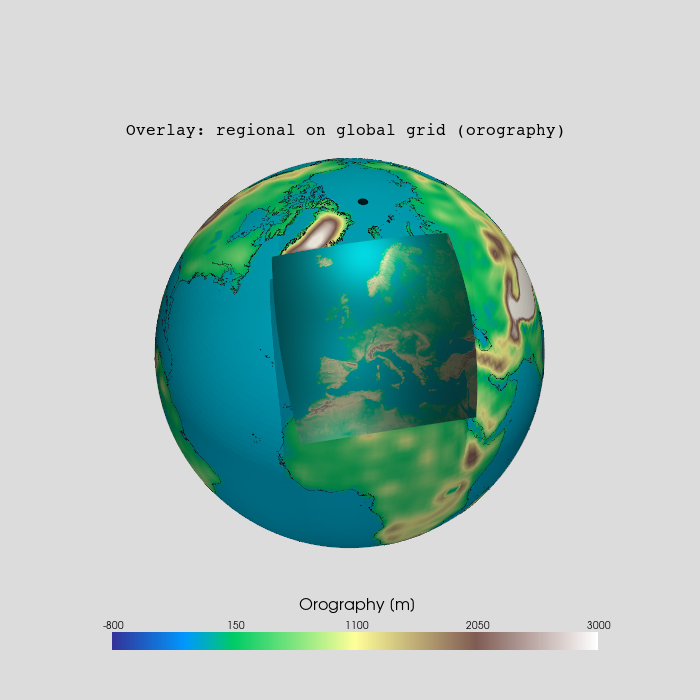
In this example, we show the overlaying of two orographies of different resolutions on the sphere. To display the orographies on a 3D sphere, we use the Python packages PyVista and GeoVista.
The global dataset is the MPI-ESM-LR orography with lower resolution on a rectilinear grid. The regional dataset is the CORDEX EUR-11 orography with higher resolution on a rotated curvilinear grid.
Content
Example data
Plotting - create mesh from 1d-coordinates - create mesh from 2d-coordinates - plot the meshes - add coastlines
Software requirements
Python 3
numpy
xarray
pyvista
geovista
Example script#
overlay_different_orography_on_sphere.py
#!/usr/bin/env python
# coding: utf-8
#
#------------------------------------------------------------------------------
#-- DKRZ example: 3D - different orographies on a sphere
#--
#-- In this example, we show the overlaying of two orographies of different
#-- resolutions on the sphere. To display the orographies on a 3D sphere, we
#-- use the Python packages PyVista and GeoVista.
#--
#-- The global dataset is the MPI-ESM-LR orography with lower resolution on a
#-- rectilinear grid. The regional dataset is the CORDEX EUR-11 orography with
#-- higher resolution on a rotated curvilinear grid.
#--
#------------------------------------------------------------------------------
#--
#-- 2026 copyright DKRZ licensed under CC BY-NC-SA 4.0
#--                 (https://creativecommons.org/licenses/by-nc-sa/4.0/deed.en)
#--
#------------------------------------------------------------------------------
import os
import pyvista as pv
from pyvista import examples
import geovista as gv
import numpy as np
import xarray as xr
import cartopy.util as cutil

#------------------------------------------------------------------------------
#-- Preliminary work
#------------------------------------------------------------------------------

#-- set title string
title = 'Overlay: regional on global grid (orography)'

#-- choose colormap
cmap = 'terrain'

#-- set data value range [m]
var_min = -800
var_max = 3000

#-- retrieve the data of the coastlines
coastlines = examples.download_coastlines()

#------------------------------------------------------------------------------
#-- Plot global MPI-ESM-LR orography on a sphere
#------------------------------------------------------------------------------

#-- First, we read the data for the Orography variable and the land-sea mask.

#-- global orography
orog_file1 = os.environ['HOME'] + '/data/CMIP5/atmos/orog_fx_MPI-ESM-LR_rcp26_r0i0p0.nc'

#-- open orography file
ds1_global = xr.open_dataset(orog_file1)
var1 = ds1_global.orog

#-- global land area fraction
laf_file1 = os.environ['HOME'] + '/data/CMIP5/atmos/sftlf_fx_MPI-ESM-LR_rcp26_r0i0p0.nc'

#-- open land-sea-mask file
ds1_mask = xr.open_dataset(laf_file1)
lsm1 = ds1_mask.sftlf.where(ds1_mask.sftlf > 0.5, ds1_mask.sftlf, 0)
land_only1 = np.where(lsm1 > 0.5, var1, -101)    #-- min contour value - 1

lat = ds1_global.lat
lon = ds1_global.lon

dlat = lat[1]-lat[0]
dlon = lon[1]-lon[0]

#-- To prevent a gap at Greenwich Meridian, we add a longitude cyclic point for
#-- Greenwich Meridian.
cyclic_data, cyclic_lon = cutil.add_cyclic_point(land_only1, coord=lon)


#------------------------------------------------------------------------------
#-- Create the mesh of the global data.
#------------------------------------------------------------------------------

#-- use the longitudes and latitudes of the input data to generate the mesh
#-- coordinates
xx, yy, zz = np.meshgrid(np.deg2rad(cyclic_lon), np.deg2rad(lat), [0])

#-- transform the input coordinates to spherical coordinates
radius = 1.
x = radius * np.cos(yy) * np.cos(xx)
y = radius * np.cos(yy) * np.sin(xx)
z = radius * np.sin(yy)

#-- Crearte a structured 3d-grid from the longitudes, latitudes, and one
#-- vertical level and add the example data.

#-- create a structured grid object
grid = pv.StructuredGrid(x, y, z)

#-- add data to the structured grid object
grid['orog1'] = cyclic_data.data.ravel(order='F')

#------------------------------------------------------------------------------
#-- Create the plot on the sphere.
#------------------------------------------------------------------------------

#-- create the plotter
plotter = gv.GeoPlotter(window_size=(800,800))

#-- add the data to the plotter
actor = plotter.add_mesh(grid,
                         cmap=cmap,
                         interpolate_before_map=False,
                         lighting=True,
                         categories=True,
                         show_scalar_bar=False)
actor.mapper.scalar_range = var_min, var_max

#-- add color bar
sbar_args = dict(interactive=False,
                 vertical=False,
                 n_labels=5,
                 title_font_size=16,
                 label_font_size=10,
                 outline=False,
                 width=0.7,
                 height=0.07,
                 position_x= 0.175,
                 position_y= 0.07,
                 fmt='{0:5.0f}')

sbar = plotter.add_scalar_bar('Orography [m]',  **sbar_args)
#-- add more space between scalar bar title and the color labels
sbar.GetTitleTextProperty().SetLineOffset(-10.)

#-- add coastlines to the plotter
actor = plotter.add_mesh(coastlines, color='black', line_width=0.5)

#-- display the result
plotter.show()

#------------------------------------------------------------------------------
#-- Plot regional CORDEX EUR-11 orography on a sphere
#------------------------------------------------------------------------------

#-- In the following, we will show how the rotated curvilinear data is handled
#-- in PyVista in order to display it on the sphere.

#-- regional orography
orog_file2 = os.environ['HOME'] + '/data/CORDEX/EUR-11/orog_EUR-11_MPI-M-MPI-ESM-LR_historical_r0i0p0_CLMcom-CCLM4-8-17_v1_fx.nc'

#-- open regional file
ds2 = xr.open_dataset(orog_file2)
var2 = ds2.orog

#-- land-sea-mask data
laf_file2 = os.environ['HOME'] + '/data/CORDEX/EUR-11/sftlf_EUR-11_MPI-M-MPI-ESM-LR_historical_r0i0p0_CLMcom-CCLM4-8-17_v1_fx.nc'

#-- open land-sea-mask data file
ds2_mask = xr.open_dataset(laf_file2)
lsm2 = ds2_mask.sftlf

#-- mask ocean
lsm2 = np.where(lsm2 > 0.5, lsm2, 0)
land_only2 = np.where(lsm2 > 0.5, var2, -101)    #-- min contour value - 1
land_only2

#------------------------------------------------------------------------------
#-- To create the mesh, we have to proceed slightly differently here, as the
#-- data is located on a rotated curvilinear grid.
#------------------------------------------------------------------------------
mesh = gv.Transform.from_2d(var2.lon,
                            var2.lat,
                            data=land_only2,
                            name=f"{var2.standard_name} / {var2.units}")

#-- remove cells from the mesh with missing values
mesh = mesh.threshold()

#------------------------------------------------------------------------------
#-- Create the plot on the sphere.
#------------------------------------------------------------------------------
plotter = gv.GeoPlotter()

sphere = pv.Sphere(radius=1.0, theta_resolution=100, phi_resolution=100)
plotter.add_mesh(sphere, color='gainsboro')

actor = plotter.add_mesh(mesh, cmap='terrain')
actor.mapper.scalar_range = var_min, var_max

plotter.add_coastlines()

plotter.camera.zoom(1.3)
cpos = plotter.camera_position

plotter.camera_position = 'yz'
plotter.camera.azimuth = 10
plotter.camera.elevation = 45   #-- move camera upward
plotter.camera.roll -= 5        #-- 'rotate' the sphere

plotter.show()

#------------------------------------------------------------------------------
#-- Combine both meshes in one plot
#------------------------------------------------------------------------------

#-- Now we have everything we need to draw both meshes on the sphere in the same
#-- plot. We also add a title string, the cell edges of the global grid, a
#-- camera, and some lighting to create a nice plot.

#----------------------------------------------------------------
#-- create the plotter
#----------------------------------------------------------------
plotter = gv.GeoPlotter(window_size=(700,700))

plotter.set_background('gainsboro')

#----------------------------------------------------------------
#-- add a title string
#----------------------------------------------------------------
plotter.add_text(title,
                 font='courier',
                 viewport=True,
                 position=(0.18, 0.8),
                 font_size=8)

#----------------------------------------------------------------
#-- add MPI-ESM-LR mesh
#----------------------------------------------------------------
actor = plotter.add_mesh(grid,
                         cmap=cmap,
                         lighting=True,
                         show_scalar_bar=False)
actor.mapper.scalar_range = var_min, var_max

#----------------------------------------------------------------
#-- add color bar
#----------------------------------------------------------------
sbar_args = dict(interactive=False,
                 vertical=False,
                 n_labels=5,
                 title_font_size=16,
                 label_font_size=10,
                 outline=False,
                 width=0.7,
                 height=0.07,
                 position_x= 0.16,
                 position_y= 0.07,
                 fmt='{0:5.0f}')
sbar = plotter.add_scalar_bar('Orography [m]',  **sbar_args)
#-- add more space between scalar bar title and the color labels
sbar.GetTitleTextProperty().SetLineOffset(-10.)

#----------------------------------------------------------------
#-- add CORDEX EUR-11 mesh
#--   - move the regional mesh up higher to make it more visible
#--     by creating shadows
#--   - change the attributes so that the applied mesh contrasts
#--     better from the one underneath
#----------------------------------------------------------------
actor = plotter.add_mesh(mesh,
                         cmap=cmap,
                         show_scalar_bar=False,
                         split_sharp_edges=True,
                         pbr=True,
                         metallic=1.0,
                         roughness=0.5,
                         zlevel=1000)
actor.mapper.scalar_range = var_min, var_max
plotter.enable_shadows()

#----------------------------------------------------------------
#-- add coastlines to the plotter
#----------------------------------------------------------------
plotter.add_coastlines()

#----------------------------------------------------------------
#-- set camera
#----------------------------------------------------------------
plotter.camera.zoom(1.3)
plotter.camera_position = 'yz'
plotter.camera.azimuth = 0
plotter.camera.elevation = 45   #-- move camera upward
plotter.camera.roll -= 5        #-- 'rotate' the sphere

#----------------------------------------------------------------
#-- light settings
#----------------------------------------------------------------
light = pv.Light()
light.set_direction_angle(0, 0)     #-- +x-direction
light.intensity = 0.25               #-- set light intensity to x%
plotter.add_light(light)

#----------------------------------------------------------------
#-- display the result and save output to PNG
#----------------------------------------------------------------
plotter.show(screenshot='plot_pyvista_grid_resolutions_overlay.png')
Plot result#