About data on curvilinear or rotated regional grids#
2D Climate data can be sampled using different grid types and topologies, which might make a difference when it comes to data analysis and visualization. As the grid lines of regular or rectilinear grids are aligned with the axes of the geopgraphical lat-lon coordinate system, these model grids are relatively easy to deal with. A common, but more complex case is that of a curvilinear or a rotated (regional) grid. In this blog article we want to illuminate this case a bit; we describe how to identify a curvilinear grid, and we demonstrate how to visualize the data using the “normal” cylindric equidistant map projection.
Data can not only be stored in different file formats (e.g. netCDF, GRIB), but also in different data structures. Besides its spatial dimension (e.g. 1D, 2D, 3D), we need to have a closer look at the grid and the topology used. As the time dependency of the data is encoded as the time dimension, a variable might be called a 3D variable although the spatial grid is only 2D.
Variables 1D (z.B. timeseries)
temp_mean(time)
Variables on a 2D grid
temp_mean(lat, lon)
temperature(time, lat, lon)
Variables on a 3D grid
temp_ymean(level, lat, lon)
temperature(time, level, lat, lon)
The most simple spatial 2D grid is a regular grid, which is characterized by perpendicular coordinate axes that are aligned with the lat-lon-coordinate system, and a regular interval between the grid points. If the values for latitude and/or longitude are ascending with varying distances, one speaks of a rectilinear grid.
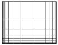
As soon as you work with data from regional models or specific ocean models, you get a different type of grid, which is often not immediately identified, unless you know what to look for. Meant is the curvilinear grid. Curvilinear grids are spatial grids whose grid points do not lie on straight lines but on curved lines. To ensure this the latitude and longitude arrays are no longer 1-dimensional, but 2-dimensional.
Rectilinear grid: 1-dimensional latitude and longitude arrays
lat(m)
lon(n)
Curvilinear grid: 2-dimensional latitude and longitude arrays
lat(m,n)
lat(m,n)
regular grid |
rectilinear grid |
curvilinear grid |

Programs like Panoply and ncview can read and display variables on curvilinear grids quickly. Programs like NCL, Python and Paraview are used to visualize the data in a more comprehensive way.
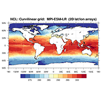
In the following example we use the sea surface temperature variable tos of a MIP-ESM-LR data set to show how an NCL and a corresponding Python script looks like.
NCL scripts#
fname = "MPI-ESM-LR_tos.nc"

cmap = read_colormap_file("MPL_RdYlBu")
cmap = cmap(::-1,:)             ;-- reverse colormap


f = addfile(fname,"r")  ;-- open file

var   = f->tos(0,:,:)           ;-- define variable
lat2d = f->lat                  ;-- get 2D latitude array
lon2d = f->lon                  ;-- get 2D longitude array

;-- open a workstation
wks_type          = "png"
wks_type@wkWidth  = 800
wks_type@wkHeight = 800
wks = gsn_open_wks(wks_type,"plot_NCL_curvilinear_MPI-ESM-LR")

;-- set plot resources
res = True                      ;-- set resources
res@gsnAddCyclic   = False      ;-- don't add lon cyclic point
res@gsnMaximize    = True       ;-- maximize plot output
res@gsnLeftString  = ""
res@gsnRightString = ""

res@cnFillOn       = True       ;-- turn on contour fill
res@cnFillPalette  = cmap
res@cnFillMode     = "CellFill" ;-- change contour fill mode
res@cnLineLabelsOn = False
res@cnLinesOn      = False      ;-- don't draw contour lines

res@tiMainString   = "NCL: Curvilinear grid:  MPI-ESM-LR  (2D lat/lon arrays)"

res@sfXArray       = lon2d      ;-- longitude grid cell center
res@sfYArray       = lat2d      ;-- latitude grid cell center

res@mpFillOn       = False
res@mpGridLineColor = "gray"
res@mpGridAndLimbOn =  True                 ;-- plot grid lines
res@mpGridLatSpacingF =  30.
res@mpGridLonSpacingF =  30.
res@mpDataBaseVersion = "MediumRes"
res@mpGeophysicalLineThicknessF = 2

plot1 = gsn_csm_contour_map(wks,var,res) ;-- create the plot
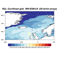
res@mpLimitMode = "LatLon"
res@mpMinLatF   =  50.           ;-- sub-region minimum latitude
res@mpMaxLatF   =  85.           ;-- sub-region maximum latitude
res@mpMinLonF   = -40.           ;-- sub-region minimum longitude
res@mpMaxLonF   =  20.           ;-- sub-region maximum longitude

res@mpGridLatSpacingF =  10.
res@mpGridLonSpacingF =  10.

plot2 = gsn_csm_contour_map(wks,var,res)   ;-- create the plot
Python scripts#
from matplotlib import cm
from matplotlib.colors import BoundaryNorm
import matplotlib.pyplot as plt
import matplotlib.ticker as mticker
from cartopy.mpl.ticker import LongitudeFormatter, LatitudeFormatter
import cartopy.crs as ccrs
import xarray as xr
import numpy as np
import copy
def main():
"""
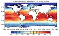
Read MPI-ESM-LR data and create a pcolormesh plot.
"""
# set projection
projection = ccrs.PlateCarree()
# set colormap
colormap = 'RdYlBu_r'
cmap = copy.copy(cm.get_cmap(colormap))
cmap.set_bad(color='white', alpha=0)
# read file
fname = 'MPI-ESM-LR_tos.nc'
ds = xr.open_dataset(fname)
# read variable tos, lat and lon
var = ds.tos.isel(time=0)
lat = ds.lat
lon = ds.lon
# fix lon data discontinuity
fixed_lon = lon.copy()
for i, start in enumerate(np.argmax(np.abs(np.diff(lon)) > 180, axis=1)):
fixed_lon[i, start+1:] += 360
# lat and lon are bounds, so var should be the value *inside* those bounds.
# Therefore, remove the last value from the var array.
var = var[:-1, :-1]
# set contour level min/max values and number of contours/colors
levels = mticker.MaxNLocator(nbins=14).tick_values(var.min(), var.max())
norm = BoundaryNorm(levels, ncolors=cmap.N, clip=True)
#var_masked = np.ma.masked_where(np.isnan(var),var)
fig = plt.figure(figsize=(8, 5))
ax = plt.axes(projection=ccrs.PlateCarree())
ax.coastlines()
ax.set_xticks(np.arange(-180,180+30,30), crs=ccrs.PlateCarree())
ax.set_yticks(np.arange(-90,90+30,30), crs=ccrs.PlateCarree())
lon_formatter = LongitudeFormatter(zero_direction_label=True)
lat_formatter = LatitudeFormatter()
ax.xaxis.set_major_formatter(lon_formatter)
ax.yaxis.set_major_formatter(lat_formatter)
gl = ax.gridlines(crs=ccrs.PlateCarree(), draw_labels=False,
linewidth=0.5, color='gray', alpha=0.5, linestyle='-')
gl.xlocator = mticker.FixedLocator(np.arange(-180,180+30,30))
gl.ylocator = mticker.FixedLocator(np.arange(-90,90+30,30))
plot = ax.pcolormesh(fixed_lon, lat, var, shading='auto', cmap=cmap, norm=norm,)
cbar = fig.colorbar(plot, ax=ax, fraction=0.13, pad=0.1,
orientation='horizontal', shrink=0.75)
cbar.solids.set_edgecolor("black")
cbar.ax.tick_params(labelsize=8)
plt.title('Py: Curvilinear grid: MPI-ESM-LR (2D lat/lon arrays)')
plt.savefig('plot_Python_curvilinear_MPI-ESM-LR_global.png', bbox_inches='tight', dpi=200)
if __name__ == "__main__":
main()
from matplotlib import cm
from matplotlib.colors import BoundaryNorm
import matplotlib.pyplot as plt
import matplotlib.ticker as mticker
from cartopy.mpl.ticker import LongitudeFormatter, LatitudeFormatter
import cartopy.crs as ccrs
import xarray as xr
import numpy as np
import copy
def main():
"""
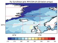
Read MPI-ESM-LR data and create a pcolormesh plot.
"""
# set projection
projection = ccrs.PlateCarree()
# set colormap
colormap = 'RdYlBu_r'
cmap = copy.copy(cm.get_cmap(colormap))
cmap.set_bad(color='white', alpha=0)
# file name
fname = 'MPI-ESM-LR_tos.nc'
# read file
ds = xr.open_dataset(fname)
# read variable tos, lat and lon
var = ds.tos.isel(time=0)
lat = ds.lat
lon = ds.lon
# fix lon data discontinuity
fixed_lon = lon.copy()
for i, start in enumerate(np.argmax(np.abs(np.diff(lon)) > 180, axis=1)):
fixed_lon[i, start+1:] += 360
# lat and lon are bounds, so var should be the value *inside* those bounds.
# Therefore, remove the last value from the var array.
var = var[:-1, :-1]
# set contour level min/max values and number of contours/colors
levels = mticker.MaxNLocator(nbins=14).tick_values(var.min(), var.max())
norm = BoundaryNorm(levels, ncolors=cmap.N, clip=True)
#var_masked = np.ma.masked_where(np.isnan(var),var)
fig = plt.figure(figsize=(8, 5))
ax = plt.axes(projection=ccrs.PlateCarree())
ax.coastlines()
ax.set_xticks(np.arange(-180,180+30,30), crs=ccrs.PlateCarree())
ax.set_yticks(np.arange(-90,90+30,30), crs=ccrs.PlateCarree())
lon_formatter = LongitudeFormatter(zero_direction_label=True)
lat_formatter = LatitudeFormatter()
ax.xaxis.set_major_formatter(lon_formatter)
ax.yaxis.set_major_formatter(lat_formatter)
gl = ax.gridlines(crs=ccrs.PlateCarree(), draw_labels=False,
linewidth=1, color='red', alpha=0.5, linestyle='-')
gl.xlocator = mticker.FixedLocator(np.arange(-180,180+30,20))
gl.ylocator = mticker.FixedLocator(np.arange(-90,90+30,10))
plot = ax.pcolormesh(fixed_lon, lat, var, shading='auto',
cmap=cmap, norm=norm, lw=0.05,
edgecolors=None)
ax.set_extent([-40, 20, 50, 85], crs=ccrs.PlateCarree())
cbar = fig.colorbar(plot, ax=ax, fraction=0.13, pad=0.1,
orientation='horizontal', shrink=0.75)
cbar.solids.set_edgecolor('k')
cbar.ax.tick_params(labelsize=8, width=0.1)
plt.title('Py: Curvilinear grid: MPI-ESM-LR (2D lat/lon arrays)')
plt.savefig('plot_Python_curvilinear_MPI-ESM-LR_zoom.png', bbox_inches='tight', dpi=200)
if __name__ == "__main__":
main()
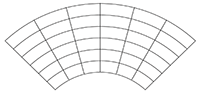
Rotated grid#
A special case is a curvilinear grid using a rotated pole (rotated grid), which is often used by regional models. In this case you have to look carefully at the dimensions, because the dimensions of the data variable seem at first sight to be defined on a regular grid, since the coordinate variables of the data variables are 1-dimensional.
E.g. for a variable tas
tas(time,rlat,rlon)
But if you look at the names of the dimensions of the data variable more precisely, they usually do not depend on lat and lon or latitude and longitude, but rather rlat and rlon.
rlat(rlat)
rlon(rlon)
With a little luck the variables lat and lon of the regular non-rotated grid are included in the file, if not, the variable rotated_pole with the attributes grid_north_pole_latitude and grid_north_pole_longitude must be included to transform the rotated to the non-rotated grid.
As an example of a curvilinear grid we use CORDEX EUR-11 data. With the command line program ‘ncdump’ we can take a look at the metadata of the file contents.
dimensions:
time = UNLIMITED ; // (12 currently)
bnds = 2 ;
rlon = 424 ;
rlat = 412 ;
variables:
double time(time) ;
time:axis = "T" ;
time:bounds = "time_bnds" ;
time:calendar = "standard" ;
time:long_name = "time" ;
time:standard_name = "time" ;
time:units = "days since 1949-12-01 00:00:00" ;
double lon(rlat, rlon) ;
lon:standard_name = "longitude" ;
lon:long_name = "longitude" ;
lon:units = "degrees_east" ;
double lat(rlat, rlon) ;
lat:standard_name = "latitude" ;
lat:long_name = "latitude" ;
lat:units = "degrees_north" ;
double time_bnds(time, bnds) ;
time_bnds:units = "days since 1949-12-01 00:00:00" ;
time_bnds:calendar = "standard" ;
float tas(time, rlat, rlon) ;
tas:standard_name = "air_temperature" ;
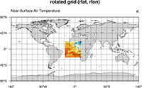
tas:long_name = "Near-Surface Air Temperature" ;
tas:units = "K" ;
tas:coordinates = "lon lat height" ;
tas:_FillValue = 1.e+20f ;
tas:missing_value = 1.e+20f ;
tas:cell_methods = "time: mean" ;
tas:grid_mapping = "rotated_pole" ;
double rlon(rlon) ;
rlon:standard_name = "grid_longitude" ;
rlon:long_name = "longitude in rotated pole grid" ;
rlon:units = "degrees" ;
rlon:axis = "X" ;
double rlat(rlat) ;
rlat:standard_name = "grid_latitude" ;
rlat:long_name = "latitude in rotated pole grid" ;
rlat:units = "degrees" ;
rlat:axis = "Y" ;
char rotated_pole ;
rotated_pole:grid_mapping_name = "rotated_latitude_longitude" ;
rotated_pole:grid_north_pole_latitude = 39.25 ;
rotated_pole:grid_north_pole_longitude = -162. ;
double height ;
height:axis = "Z" ;
height:long_name = "height" ;
height:positive = "up" ;
height:standard_name = "height" ;
height:units = "m" ;
If you read the metadata carefully, you will quickly see that
the data variable tas
depends on rlat and rlon
has the attribute coordinates which refers to lat and lon (and height)
has the attribute grid_mapping which refers to the variable rotated_pole
the coordinate variables rlat and rlon
are 1-dimensional
refer to a rotated pole grid
the variable lon and lat
are 2-dimensional
the variable rotated_pole
has the attribute grid_north_pole_latitude
has the attribute grid_north_pole_longitude
Now we know that the data are in the region of Europe, but if you look at the assigned latitudes (rlat) and longitudes (rlon), you quickly notice that they are rather above Africa. With CDO’s sinfo operator we can see both, the rotated and the non-rotated coordinate variable values (if included in the file).
cdo sinfon CORDEX_EUR-11.nc
   File format : NetCDF4 classic zip
    -1 : Institut Source   T Steptype Levels Num    Points Num Dtype : Parameter name
     1 : unknown  unknown  v instant       1   1    174688   1  F32z : tas
   Grid coordinates :
     1 : curvilinear              : points=174688 (424x412)
                              lon : -44.59386 to 64.96438 degrees_east
                              lat : 21.98783 to 72.585 degrees_north
                          mapping : rotated_latitude_longitude
                             rlon : -28.375 to 18.155 by 0.11 degrees
                             rlat : -23.375 to 21.835 by 0.11 degrees
   Vertical coordinates :
     1 : height                   : levels=1  scalar
                           height : 2 m
   Time coordinate :  12 steps
     RefTime =  1949-12-01 00:00:00  Units = days  Calendar = standard  Bounds = true
  YYYY-MM-DD hh:mm:ss  YYYY-MM-DD hh:mm:ss  YYYY-MM-DD hh:mm:ss  YYYY-MM-DD hh:mm:ss
  1970-01-16 12:00:00  1970-02-15 00:00:00  1970-03-16 12:00:00  1970-04-16 00:00:00
  1970-05-16 12:00:00  1970-06-16 00:00:00  1970-07-16 12:00:00  1970-08-16 12:00:00
  1970-09-16 00:00:00  1970-10-16 12:00:00  1970-11-16 00:00:00  1970-12-16 12:00:00
In the following NCL and Python with Matplotlib/Cartopy are used to visualize the CORDEX EUR-11 near-surface air temperature data with a cylindrical equidistant map projection.
A. NCL
The first script uses NCL with its easiest way to plot the rotated data using the lat and lon variables instead of rlat and rlon.
;-- open file and read variables
fname = "CORDEX_EUR-11_tas.nc"
f    = addfile(fname,"r")
var  = f->tas(0,:,:)
lat = f->lat
lon = f->lon

var@lat2d = lat    ;-- tell NCL to use the 2D lat and lon variables
var@lon2d = lon

minlat = min(var@lat2d)                 ;-- retrieve minimum latitude value
minlon = min(var@lon2d)                 ;-- retrieve maximum latitude value
maxlat = max(var@lat2d)                 ;-- retrieve minimum longitude value
maxlon = max(var@lon2d)                 ;-- retrieve maximum longitude value

;-- open a workstation
wks = gsn_open_wks("png","plot_NCL_curvilinear_grid_derotated_1")

;-- set resources
res                   = True
res@gsnAddCyclic      = False           ;-- don't add lon cyclic point

res@mpDataBaseVersion = "MediumRes"     ;-- choose map database
res@mpGridAndLimbOn   = True            ;-- turn on grid lines
res@mpMinLatF         = minlat - 1.     ;-- set min lat
res@mpMaxLatF         = maxlat + 1.     ;-- set max lat
res@mpMinLonF         = minlon - 1.     ;-- set min lon
res@mpMaxLonF         = maxlon + 1.     ;-- set max lon

res@cnFillOn          = True            ;-- turn on contour fill
res@cnLinesOn         = False           ;-- don't draw contour lines
res@cnLineLabelsOn    = False
res@cnFillPalette     = "BlueYellowRed" ;-- choose colormap

res@lbLabelBarOn      = False           ;-- turn on labelbar

res@tiMainString      = "derotated grid (lat,lon)"
res@tiMainOffsetYF    = -0.03           ;-- move title downward

plot = gsn_csm_contour_map(wks, var, res)
If the variables lat and lon are not stored in the dataset the NCL script below demonstrate how to compute them to plot the data on the regular non-rotated grid. The script produces the same plot as above.
;-- set global constants
pi      =  4.0*atan(1.)
deg2rad =  pi/180.
rad2deg =  45./atan(1.)
fillval = -99999.9

;------------------------------------------------------------
;-- Function:     unrot_lon(rotlat,rotlon,pollat,pollon)
;-- Description:  transform rotated longitude to longitude
;------------------------------------------------------------
undef("unrot_lon")
function unrot_lon( rotlat:numeric, rotlon:numeric, pollat[1]:numeric, pollon[1]:numeric )
local rotlat, rotlon, nrlat, nrlon, nrlat_rank, nrlon_rank, pollon, pollat, \
      lon, s1, c1, s2, c2, rlo, rla, i, tmp1, tmp2
begin
  lon = fillval
  lon@_FillValue = fillval

  nrlat      = dimsizes(rotlat)
  nrlon      = dimsizes(rotlon)
  nrlat_rank = dimsizes(nrlat)
  nrlon_rank = dimsizes(nrlon)

  if(any(nrlat .ne. nrlon) .and. (nrlat_rank.ne.1 .or. nrlon_rank.ne.1)) then
      print("Function unrot_lon: unrot_lon:  rotlat and rotlon dimensions do not match")
    return(lon)
  end if

  if(nrlat_rank.eq.1 .and. nrlon_rank.eq.1) then
    rla = conform_dims((/nrlat,nrlon/),rotlat,0) ;-- create 2D latitude array
    rlo = conform_dims((/nrlat,nrlon/),rotlon,1) ;-- create 2D longitude array
  else
    rla = rotlat
    rlo = rotlon
  end if

  rla = rla*deg2rad                         ;-- convert from degree to radians
  rlo = rlo*deg2rad                         ;-- convert from degree to radians

  lon := (/rlo/)                            ;-- reassign lon
  lon@_FillValue=fillval

  s1 = sin(pollat*deg2rad)
  c1 = cos(pollat*deg2rad)
  s2 = sin(pollon*deg2rad)
  c2 = cos(pollon*deg2rad)

  tmp1 = s2*(-s1*cos(rlo)*cos(rla)+c1*sin(rla))-c2*sin(rlo)*cos(rla)
  tmp2 = c2*(-s1*cos(rlo)*cos(rla)+c1*sin(rla))+s2*sin(rlo)*cos(rla)

  lon = atan(tmp1/tmp2)*rad2deg

  lon@units = "degrees_east"
  print("Function unrot_lon: min/max     "+sprintf("%8.4f", min(lon(0,:)))+\
        "  "+sprintf("%8.4f", max(lon(0,:))))

  delete([/rlo,rlo,c1,s1,c2,s2,tmp1,tmp2/])

  return(lon)
end

;------------------------------------------------------------
;-- Function:     unrot_lat(rotlat,rotlon,pollat,pollon)
;-- Description:  transform rotated latitude to latitude
;------------------------------------------------------------
undef("unrot_lat")
function unrot_lat( rotlat:numeric, rotlon:numeric, pollat[1]:numeric, pollon[1]:numeric )
local rotlat, rotlon, nrlat, nrlon, nrlat_rank, nrlon_rank, pollon, pollat, \
      lat, s1, c1, rlo, rla, i
begin
  lat = fillval
  lat@_FillValue = fillval

  nrlat      = dimsizes(rotlat)
  nrlon      = dimsizes(rotlon)
  nrlat_rank = dimsizes(nrlat)
  nrlon_rank = dimsizes(nrlon)

  if(any(nrlat .ne. nrlon) .and. (nrlat_rank.ne.1 .or. nrlon_rank.ne.1)) then
    print("Function unrot_lat:  rotlat and rotlon dimensions do not match")
    return(lat)
  end if

  if(nrlat_rank.eq.1 .and. nrlon_rank.eq.1) then
    rla = conform_dims((/nrlat,nrlon/),rotlat,0) ;-- create 2D latitude array
    rlo = conform_dims((/nrlat,nrlon/),rotlon,1) ;-- create 2D longitude array
  else
    rla = rotlat
    rlo = rotlon
  end if

  rla = rla*deg2rad                         ;-- convert from degree to radians
  rlo = rlo*deg2rad                         ;-- convert from degree to radians

  lat := (/rla/)                            ;-- reassign lat
  lat@_FillValue=fillval

  s1 = sin(pollat*deg2rad)
  c1 = cos(pollat*deg2rad)

  lat = s1*sin(rla)+c1*cos(rla)*cos(rlo)
  lat = asin(lat)*rad2deg

  lat@units = "degrees_north"
  print("Function unrot_lat: min/max     "+sprintf("%8.4f", min(lat(:,0)))+\
        "  "+sprintf("%8.4f", max(lat(:,0))))

  delete([/rlo,rla,c1,s1/])

  return(lat)
end

;----------------
;  MAIN
;----------------
begin
;-- open file and read variables
  fname = "CORDEX_EUR-11_tas.nc"
  f    = addfile(fname,"r")
  var  = f->tas(0,:,:)
  rlat = f->rlat
  rlon = f->rlon

  var&rlat@units = "degrees_north"
  var&rlon@units = "degrees_east"

;-- unrotate the grid and set 2D lat/lons
  rotpole = f->rotated_pole
  pollat  = rotpole@grid_north_pole_latitude
  pollon  = rotpole@grid_north_pole_longitude

  lon2d = unrot_lon(rlat, rlon, pollat, pollon)
  lat2d = unrot_lat(rlat, rlon, pollat, pollon)

;-- define variable on unrotated grid
  var_unrot = var
  var_unrot@lon2d = lon2d
  var_unrot@lat2d = lat2d

  minlat = min(var_unrot@lat2d)             ;-- retrieve minimum latitude value
  minlon = min(var_unrot@lon2d)             ;-- retrieve maximum latitude value
  maxlat = max(var_unrot@lat2d)             ;-- retrieve minimum longitude value
  maxlon = max(var_unrot@lon2d)             ;-- retrieve maximum longitude value

;-- open a workstation
  wks = gsn_open_wks("png","plot_NCL_curvilinear_grid_derotated_2")

;-- set resources
  res                   = True
  res@gsnAddCyclic      = False             ;-- don't add lon cyclic point

  res@mpDataBaseVersion = "MediumRes"       ;-- choose map database
  res@mpGridAndLimbOn   = True              ;-- turn on grid lines
  res@mpMinLatF         = minlat - 1.       ;-- set min lat
  res@mpMaxLatF         = maxlat + 1.       ;-- set max lat
  res@mpMinLonF         = minlon - 1.       ;-- set min lon
  res@mpMaxLonF         = maxlon + 1.       ;-- set max lon

  res@cnFillOn          = True              ;-- turn on contour fill
  res@cnLinesOn         = False             ;-- don't draw contour lines
  res@cnLineLabelsOn    = False
  res@cnFillPalette     = "BlueYellowRed"   ;-- choose colormap

  res@lbLabelBarOn      = False             ;-- turn on labelbar

  res@tiMainString      = "de-rotated grid (rlat, rlon)"

  plot = gsn_csm_contour_map(wks, var_unrot, res)  ;-- draw second plot

end
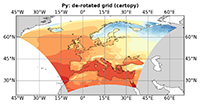
B. Python (matplotlib/cartopy)
For the use of Python cartopy provides the function RotatedPole which to the transformation from the rlat and rlon coordinate variables to the non-rotated grid.

import xarray as xr
import numpy as np
import os, sys
import matplotlib.pyplot as plt
import cartopy
import cartopy.crs as ccrs

def read_data(file_name):
    """
    Read netcdf file and return arrays: lat, lon, var, pole_longitude, pole_latitude.
    """
    ds = xr.open_dataset(file_name)
    var  = ds.tas[0,:,:]
    rlat = ds.rlat[:]
    rlon = ds.rlon[:]
    pole = ds.rotated_pole

    try:
        if hasattr(pole,'grid_north_pole_longitude'):
            px = pole.attrs['grid_north_pole_longitude']
        if hasattr(pole,'grid_north_pole_latitude'):
            py = pole.attrs['grid_north_pole_latitude']
    except:
        print('Unexpected error:', sys.exc_info()[0])
        raise

    return rlon, rlat, var, px, py

def main():
    """
    Main function.
    """
    colormap = "RdYlBu_r"

    fname = 'CORDEX_EUR-11_tas.nc'

    # read file content and return relevant variables
    rlon, rlat, var, pole_lon, pole_lat = read_data(fname)

    ax = plt.axes(projection=ccrs.PlateCarree())
    ax.set_global()
    ax.set_extent([-46, 70, 20, 75], crs=ccrs.PlateCarree())
    ax.add_feature(cartopy.feature.OCEAN, color='white', zorder=0)
    ax.add_feature(cartopy.feature.LAND, color='lightgray',zorder=0,
                   linewidth=0.5, edgecolor='black')
    ax.gridlines(draw_labels=True, linewidth=0.5, color='gray',
                 xlocs=range(-180,180,15), ylocs=range(-90,90,15))
    ax.coastlines(resolution='50m', linewidth=0.3, color='black')
    ax.set_title('Py: de-rotated grid (cartopy)', fontsize=10, fontweight='bold')

    crs = ccrs.RotatedPole(pole_longitude=pole_lon, pole_latitude=pole_lat)
    ax.contourf(rlon, rlat, var, levels=15, cmap=colormap, transform=crs)

    plt.savefig('plot_Python_curvilinear_grid_derotated_1.png', bbox_inches='tight', dpi=200)

if __name__ == '__main__':
    main()
But as already shown for NCL, here we will also give you the Python script that computes the lat and lon variables if they are missing in the file.
import xarray as xr
import numpy as np
import os, sys
import matplotlib.pyplot as plt
import cartopy
import cartopy.crs as ccrs

def read_data(file_name):
    """
    Read netcdf file and return arrays: lat, lon, var.
    """
    ds = xr.open_dataset(file_name)
    var  = ds.tas[0,:,:]
    rlat = ds.rlat[:]
    rlon = ds.rlon[:]
    pole = ds.rotated_pole

    try:
        if hasattr(pole,'grid_north_pole_longitude'):
            px = pole.attrs['grid_north_pole_longitude']
        if hasattr(pole,'grid_north_pole_latitude'):
            py = pole.attrs['grid_north_pole_latitude']
    except:
        print('Unexpected error:', sys.exc_info()[0])
        raise

    return rlon, rlat, var, px, py

def unrot_lon(rlat, rlon, pole_lat, pole_lon):
    """
    Transform rotated longitude to regular non-rotated longitude lon(2D).
    """
    nrlat = np.shape(rlat)
    nrlon = np.shape(rlon)

    nrlat_rank = np.ndim(nrlat)
    nrlon_rank = np.ndim(nrlon)

    if(np.any(nrlat != nrlon) and (nrlat_rank != 1 or nrlon_rank != 1)):
        print("Function unrot_lon: rlat and rlon dimensions do not match")
        exit()

    if(nrlat_rank == 1 and nrlon_rank == 1):
        rlo = np.tile(rlon, (nrlat[0],1))
        rla = np.transpose([rlat]*nrlon[0])
    else:
        rla = rlat
        rlo = rlon

    rla = np.deg2rad(rla)
    rlo = np.deg2rad(rlo)

    s1 = np.sin(np.deg2rad(pole_lat))
    c1 = np.cos(np.deg2rad(pole_lat))
    s2 = np.sin(np.deg2rad(pole_lon))
    c2 = np.cos(np.deg2rad(pole_lon))

    tmp1 = s2*(-s1*np.cos(rlo)*np.cos(rla)+c1*np.sin(rla))-c2*np.sin(rlo)*np.cos(rla)
    tmp2 = c2*(-s1*np.cos(rlo)*np.cos(rla)+c1*np.sin(rla))+s2*np.sin(rlo)*np.cos(rla)

    lon = np.rad2deg(np.arctan(tmp1/tmp2))

    print('Function unrot_lon: min/max  %f / %f' % (np.min(lon[0,:]), np.max(lon[0,:])) )

    return lon

def unrot_lat(rlat, rlon, pole_lat, pole_lon):
    """
    Transform rotated latitude to regular non-rotated latitude lat(2D)
    """
    nrlat = np.shape(rlat)
    nrlon = np.shape(rlon)

    nrlat_rank = np.ndim(nrlat)
    nrlon_rank = np.ndim(nrlon)

    if(np.any(nrlat != nrlon) and (nrlat_rank != 1 or nrlon_rank != 1)):
        print("Function unrot_lat: rlat and rlon dimensions do not match")
        exit()

    if(nrlat_rank == 1 and nrlon_rank == 1):
        rlo = np.tile(rlon, (nrlat[0],1))
        rla = np.transpose([rlat]*nrlon[0])
    else:
        rla = rlat
        rlo = rlon

    rla = np.deg2rad(rla)
    rlo = np.deg2rad(rlo)

    s1 = np.sin(np.deg2rad(pole_lat))
    c1 = np.cos(np.deg2rad(pole_lat))

    lat = s1*np.sin(rla)+c1*np.cos(rla)*np.cos(rlo)
    lat = np.rad2deg(np.arcsin(lat))

    print('Function unrot_lat: min/max  %f / %f' % (np.min(lat[0,:]), np.max(lat[0,:])) )

    return lat

def main():
    """
    Main function. Compute lat and lon on non-rotated grid.
    """
    colormap = "RdYlBu_r"

    dir_name = '/Users/k204045/data/CORDEX/EUR-11/'
    file_name = 'tas_EUR-11_CNRM-CERFACS-CNRM-CM5_historical_r1i1p1_SMHI-RCA4_v1_mon_197001-197012.nc'
    fname = os.path.join(dir_name,file_name)

    # read file content and return relevant variables
    rlon, rlat, var, pole_lon, pole_lat = read_data(fname)

    lon = unrot_lon(rlat, rlon, pole_lat, pole_lon)
    lat = unrot_lat(rlat, rlon, pole_lat, pole_lon)

    ax = plt.axes(projection=ccrs.PlateCarree())
    ax.set_global()
    ax.set_extent([-46, 70, 20, 75], crs=ccrs.PlateCarree())
    ax.add_feature(cartopy.feature.OCEAN, color='white', zorder=0)
    ax.add_feature(cartopy.feature.LAND, color='lightgray',zorder=0,
                   linewidth=0.5, edgecolor='black')
    ax.gridlines(draw_labels=True, linewidth=0.5, color='gray', xlocs=range(-180,180,15), ylocs=range(-90,90,15))
    ax.coastlines(resolution='50m', linewidth=0.3, color='black')
    ax.set_title('Py: de-rotated grid (cartopy)', fontsize=10, fontweight='bold')

    crs = ccrs.RotatedPole(pole_longitude=pole_lon, pole_latitude=pole_lat)
    ax.contourf(rlon, rlat, var, levels=15, cmap=colormap, transform=crs)

    plt.savefig('plot_Python_curvilinear_grid_derotated_2.png', bbox_inches='tight', dpi=200)

if __name__ == '__main__':
    main()
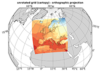
And if we choose the Orthographic map projection instead of PlateCarree the plot looks like