Isosurfaces and isocontours in regular lat-lon data#
As a map background, we use variable z_ifc extruded by the Calculator and colored by color_surface.json as in state file land_surface.pvsm. Variable clw (specific cloud water content) is made to look like fluffy clouds by using volume rendering and transparency. In a second step, we generate isosurfaces of cli (specific cloud ice content) and qr (rain mixing ratio) to get a feel for the spatial distribution and temporal evolution of cloud ice and rain. In addition to the three-dimensional isosurfaces, we then also create a vertical slice, i.e. a cross-section of the cloud ice distribution, and display isocontours for several discrete values of cli.
Isosurfaces of cloud ice and rain with volume rendering of clouds#
Note
Data directory: /work/kv0653/ParaView-Workshop/HDCP2/
Data files: hdcp2_clw.nc, hdcp2_cli.nc, hdcp2_qr.nc
State file for land background: land_surface.pvsm
Height data file: surface_1.nc
Colormap: color_clw.json
Area: HD(CP)² study area Germany (DOM02)
Steps#
Load map background
File -> Load state… -> land_surface.pvsm
Check that the path to surface_1.nc in window Fix Paths in State file is correct
Press OK
In the toolbar, press Set view direction to –Z.
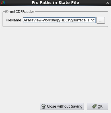
Figure 1: Fix Paths in State File
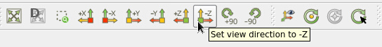
Figure 2: Set view direction to -Z
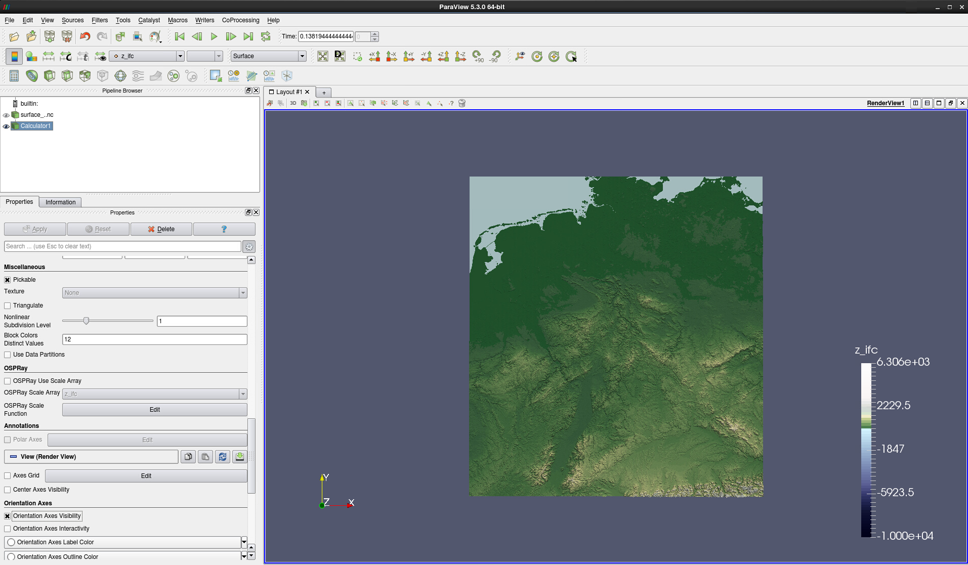
Figure 3: land_surface.pvsm : Calculator extrusion of data surface_1.nc
Load clw data by: File -> Open… -> hdcp2_clw.nc -> OK
Select NetCDF files generic and CF conventions (see Fig. 4) -> OK
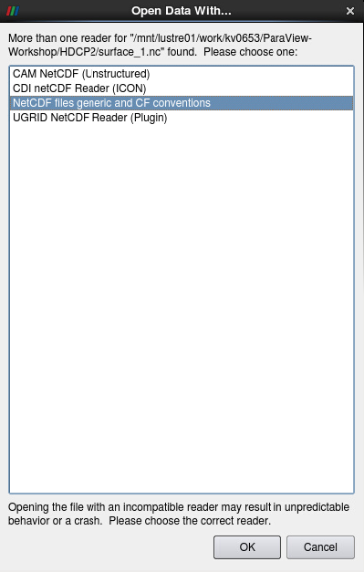
Figure 4: Select NetCDF reader
In the Properties of hdcp2_clw.nc:
Uncheck spherical coordinates
Select Output Type Image (i.e. data on a regular grid)
Hit Apply
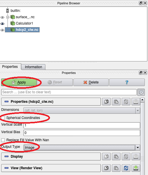
Figure 5: Applying data set hdcp2_clw.nc
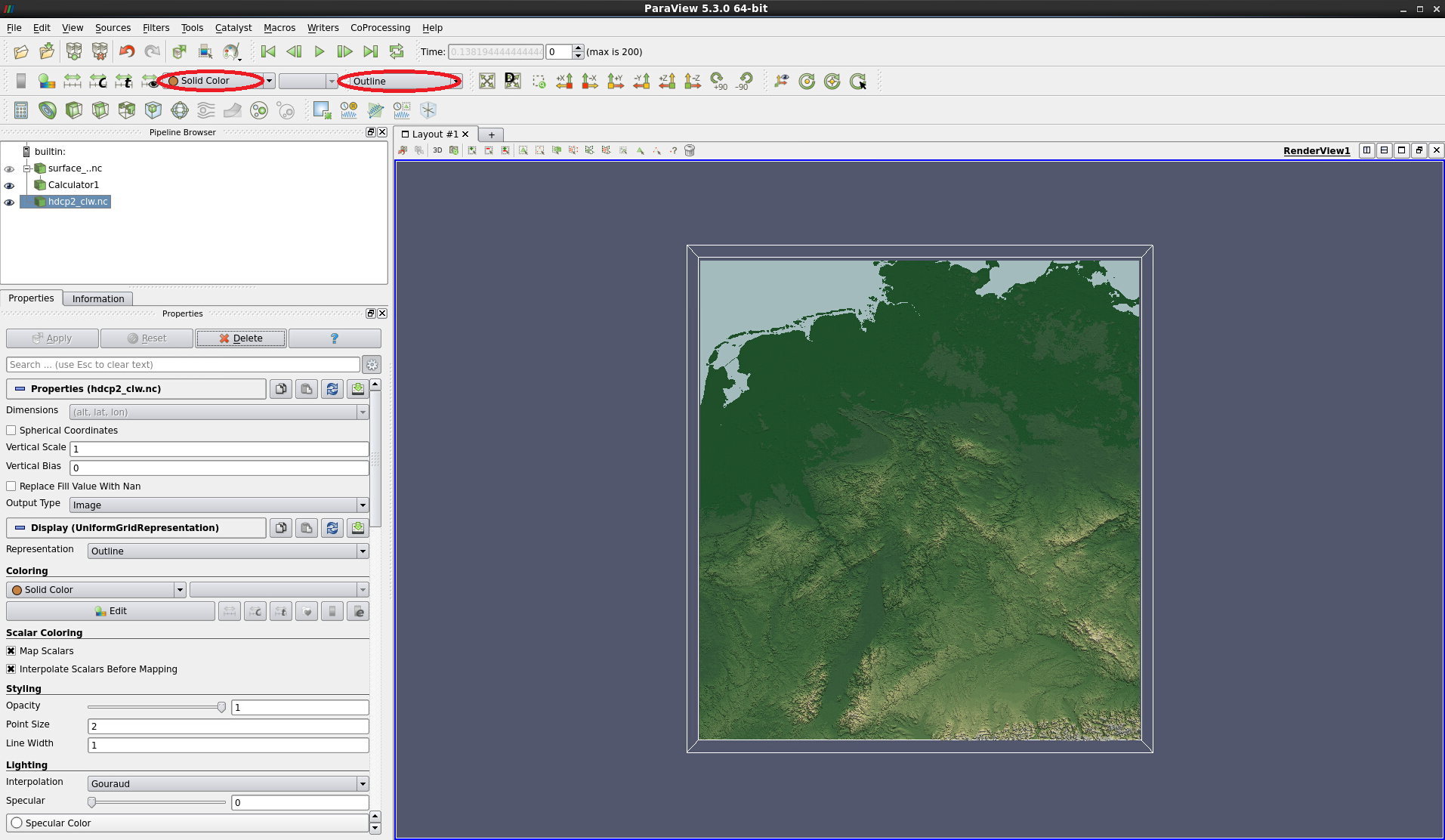
Figure 6: Data set hdcp2_clw.nc applied. Solid color and Outline (white bounding box) are default representations.
Click on the Information tab next to Properties to see information about the data set such as variables and data ranges, numbers of grid points and bounds, time steps and indices etc. (see Fig. 7)
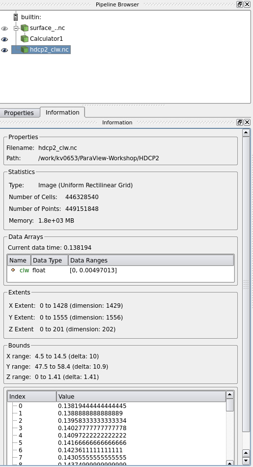
Figure 7: Information on data set hdcp2_clw.nc
This data set contains one point variable, clw, on a uniform rectilinear grid of size 1428 x 1555 x 201, extending from 47.5 to 58.4° north and from 4.5 to 14.5° east. There are 200 time steps, each of which takes up approx. 1.8 GB of memory. The current time step is 0, and the corresponding data ranges for this time step are a minimum of 0 and a maximum of 0.00497013.
In the toolbar, select the point variable clw instead of Solid Color
Change the representation from Outline to Surface
With the left mouse button pressed, click into the viewer and move your mouse cursor upwards to change the viewing angle. Your viewer should look similar to Fig. 8.
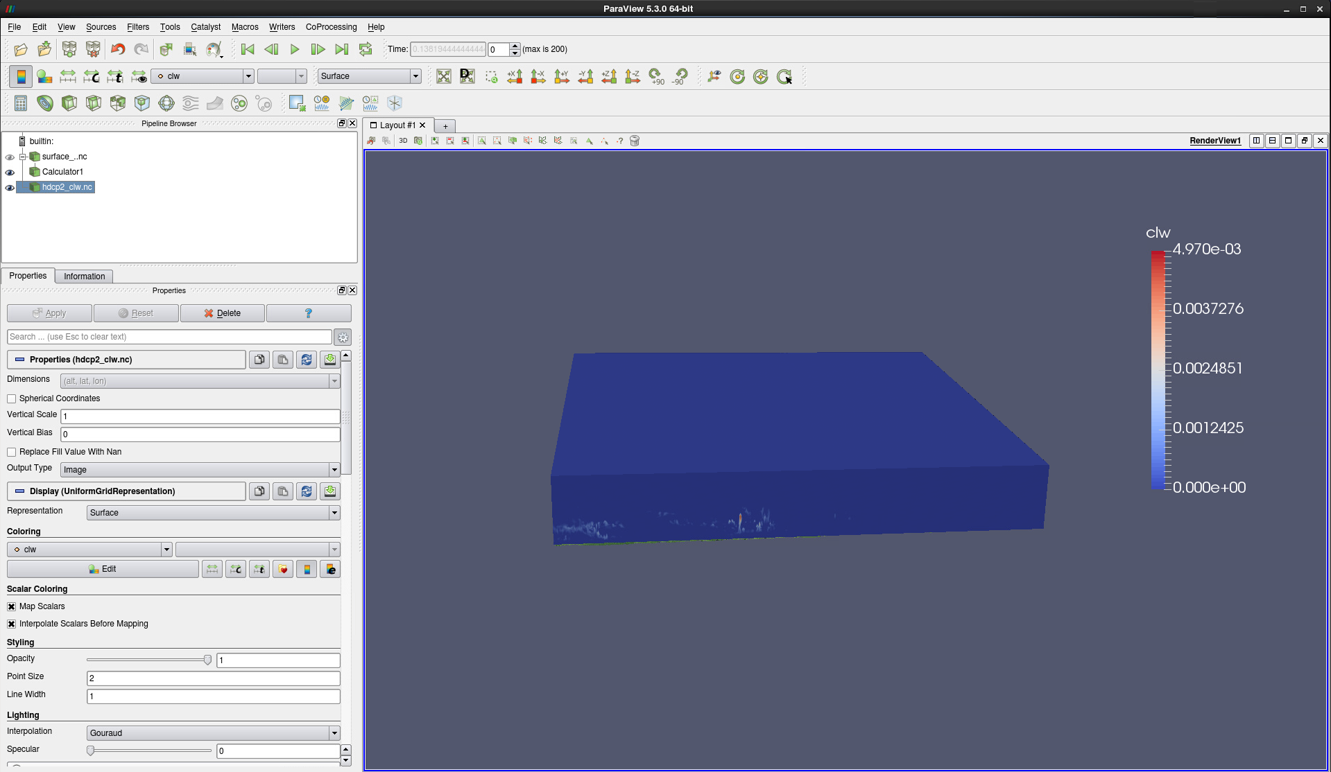
Figure 8: clw displayed as surface representation
With the surface representation, most of the areas with high cloud water content remain hidden inside the 3D volume. Volume rendering, which is a bit like ‘color by numbers’ in 3D with transparency involved, is a good choice for obtaining a more realistic representation of clouds from this data set. In contrast to large data sets on the original ICON grid, which require additional data reduction steps to interact fluently with volume rendering data, the resampled lat-lon data can readily be displayed as volume.
Change the representation to Volume.
Try different viewing angles and zoom stages to explore the data. Compare with Fig. 9.
To inspect the current opacity curve and / or edit the current colormap, invoke the Color Map Editor by clicking on the Edit Color Map button in the Coloring section (see Fig. 10)
Click on Choose preset (folder symbol with a heart) to select a more suitable colormap with shades of white and gray. The button is available in both the Coloring section and in the Color Map Editor (see Figs. 9 & 10).
Press the Import button in the newly emerged Choose Preset window.
Navigate to the colormap color_clw.json. -> click OK -> click Import, then Close. Compare with Fig. 12.
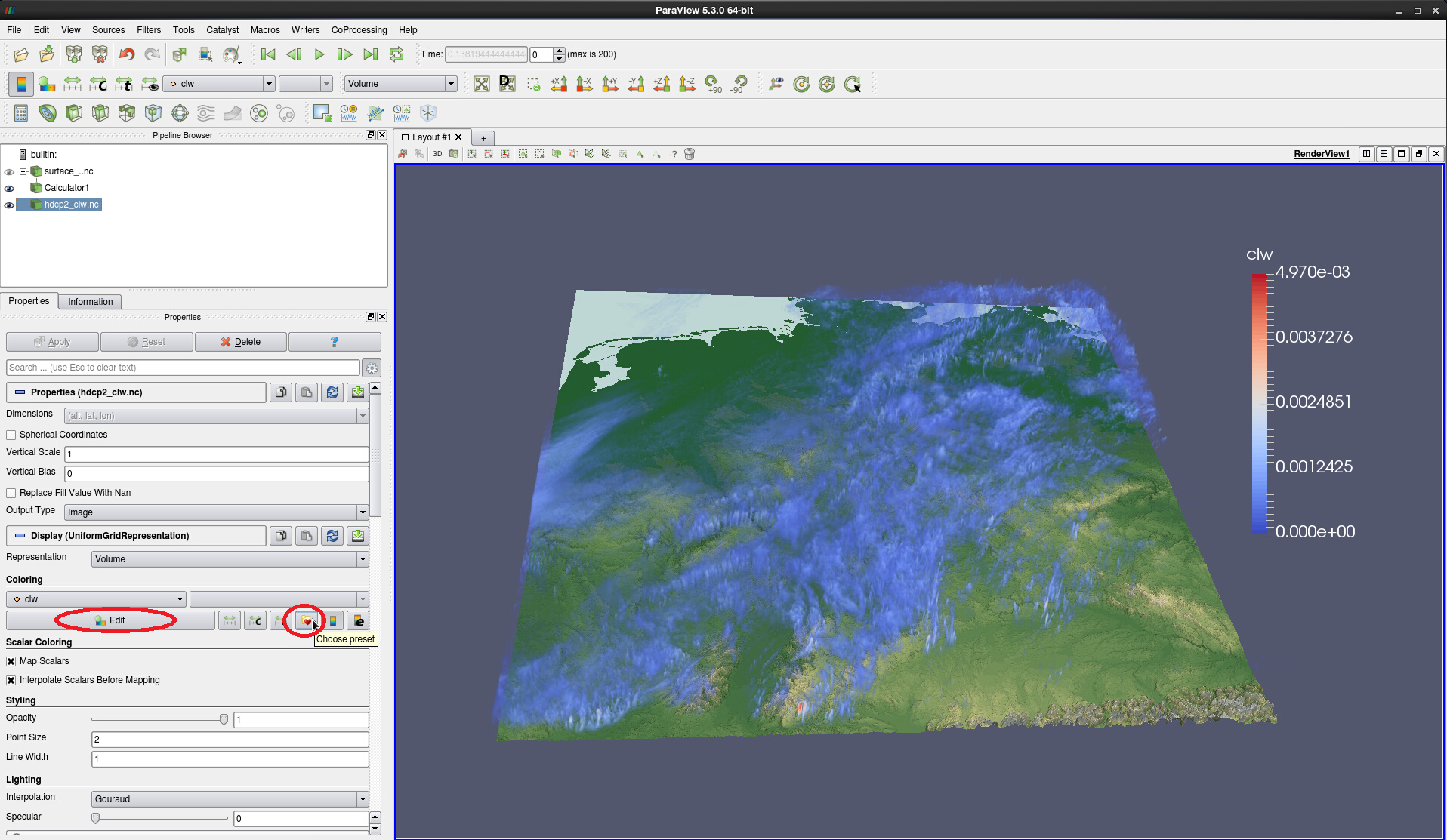
Figure 9: clw displayed as volume
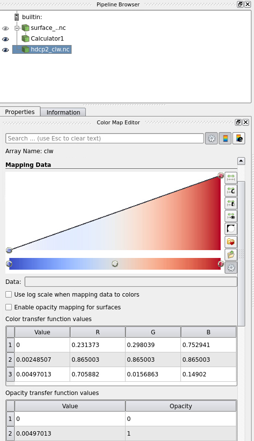
Figure 10: Color Map Editor showing the opacity curve, as well as color transfer function and opacity values.
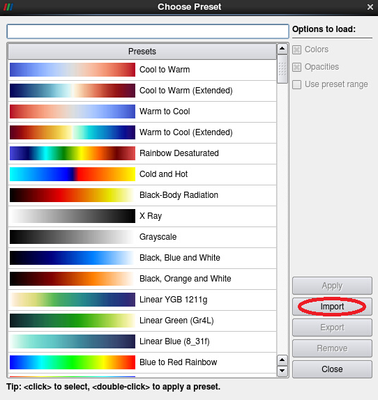
Figure 11: Import colormap preset
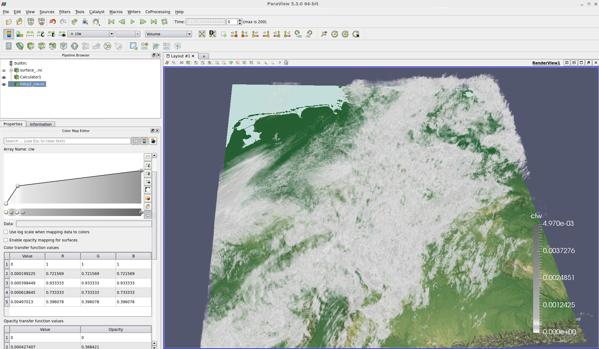
Figure 12: color_clw.json applied and opened in Color Map Editor
Repeat steps 2 to 5, this time loading hdcp2_cli.nc.
With hdcp2_cli.nc selected, press the Contour button in the Filters (see Fig. 13).
In the Contour1 properties, go to the Isosurfaces. Double-click into the first entry of the table below Value Range, overwrite it with 0.0002 and click Apply.
After a few seconds, you will see the white isosurface depicted in Fig. 14. This isosurface is drawn at the specific cloud ice content (cli) value of 0.0002 and encompasses higher values. For convenience, we have switched off the clw colormap legend by clicking on the simple colormap symbol (Toggle Color Legend Visibility) while hdcp2_clw.nc is selected in the Pipeline Browser.
In a next step, we are going to change the color of the isosurface for better visibility.
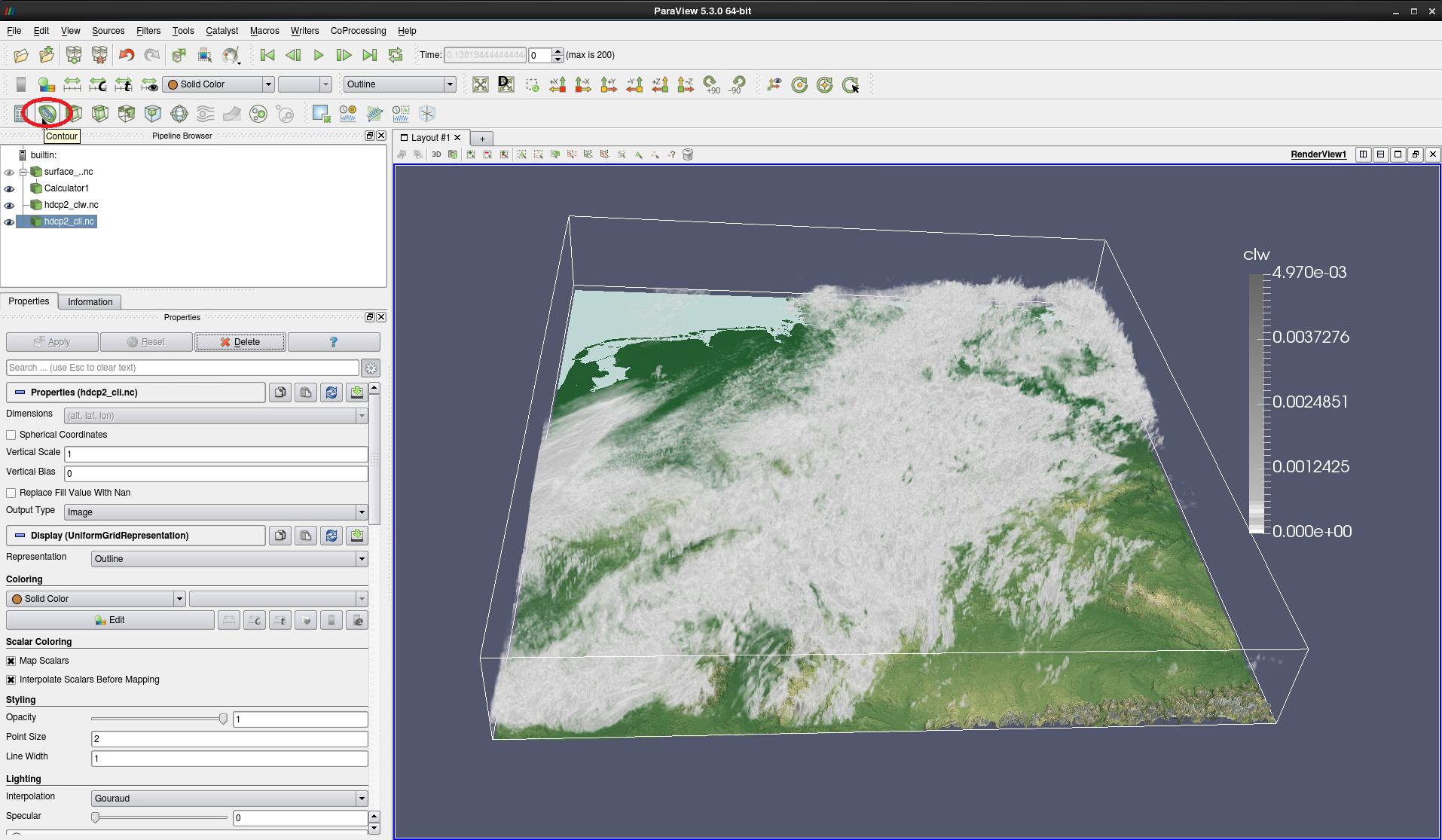
Figure 13: Selecting the Contour filter for data set hdcp2_cli.nc.
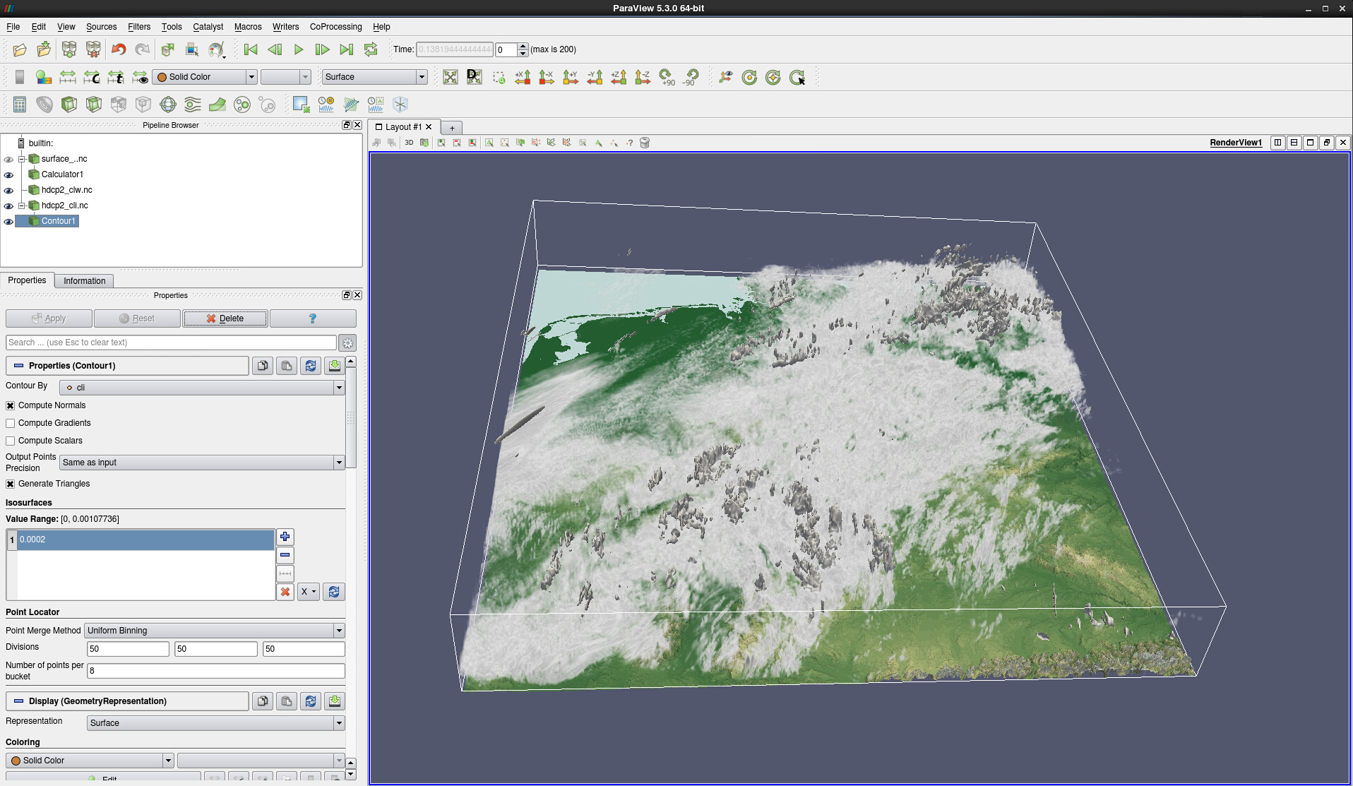
Figure 14: Isosurface at 0.0002 created by Contour filter for hdcp2_cli.nc
In the Coloring section, keep Solid Color and click on the Edit Color Map button. This calls up the Pick Solid Color dialogue window depicted in Fig. 15. You may want to choose a light pink color by clicking on one of the basic colors and subsequently modifying the color by means of the black cross and the brightness slider.

Figure 15: Picking a solid color for the cli isosurface
Repeat steps 15 to 18 for the rain mixing ratio qr in file hdcp2_qr.nc. Choose an isosurface value of 0.00014 and a lighter shade of blue to visualize rain. Compare Fig. 16.
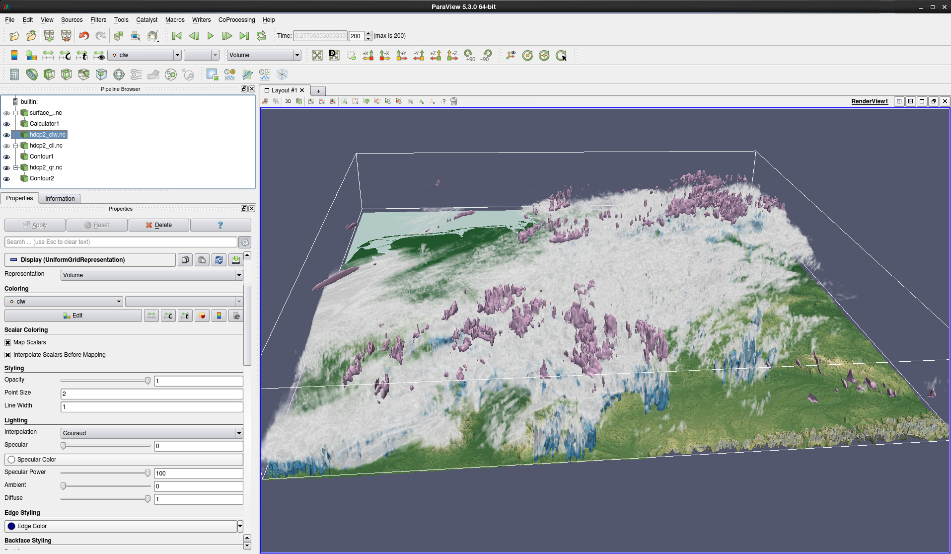
Figure 16: Volume rendering of clw and isosurfaces of cli at 0.0002 (light pink) and qr at 0.00014 (blue).
To save your visualization project, go to File -> Save State… Navigate to a directory where you have write access (e.g. your home directory on Mistral) and save the state as a .pvsm file. Have a look at the how-to on animations to learn how to create a movie for a subset of the data and its evolution over time.
Vertical contour slice of cloud ice (cli)#
In the previous example we created an isosurface, which allowed us to distinguish cli values of 0.0002 and above by drawing a surface for values of 0.0002. To get a feel for the vertica distribution of cloud ice in the atmosphere, we will now use a subset of the data and add a vertical cross-section (i.e. a slice) and add iscontours for several discrete values of cli.
We suggest that you start with your saved state from above and save it with a different name. For now you may switch off the visualization of qr by clicking on the black eye symbol to the left of Contour2 in the Pipeline Browser. However, we suggest that you keep this data source loaded to reuse the state file later on for creating a time animation of rain, clouds and cloud ice.
We start with a project that looks like this:
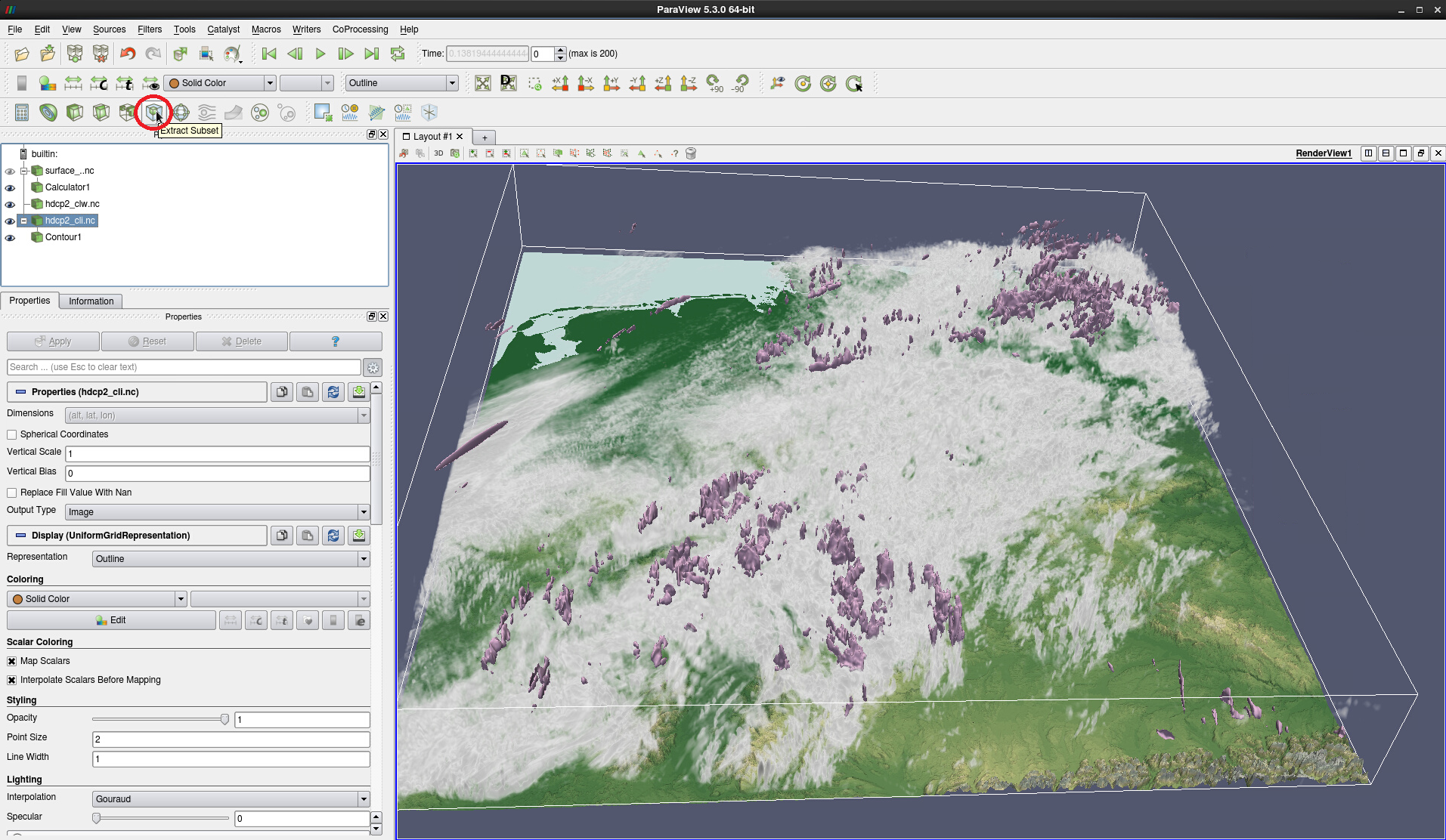
Figure 17: Volume rendering of clw and isosurfaces of cli at 0.0002 withExtract Subsetfilter highlighted
- The next steps are as follows:
Select data source hdcp2_cli.nc in the Pipeline Browser
Click on the Extract Subset filter in the toolbar (see Fig. 17)
In the Properties of ExtractSubset1, fill the VOI (Volume Of Interest) fields as follows:
Click Apply
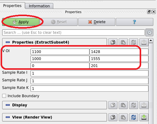
Figure 18: Properties of ExtractSubset1
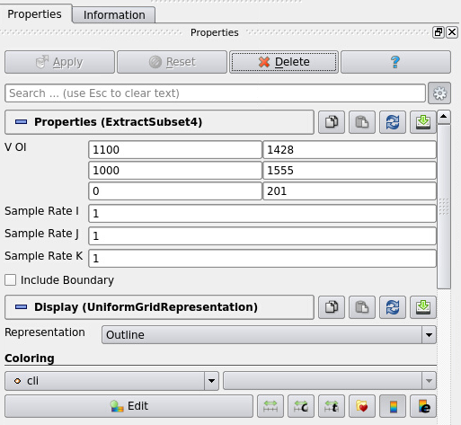
Figure 19: Properties of ExtractSubset1 after clicking Apply
Clicking Apply has changed the Properties of ExtractSubset1 according to Fig. 19. The subset of cli is now displayed as Outline, i.e. as a smaller, white-rimmed box in the northeastern corner of the data domain (see Fig. 20).
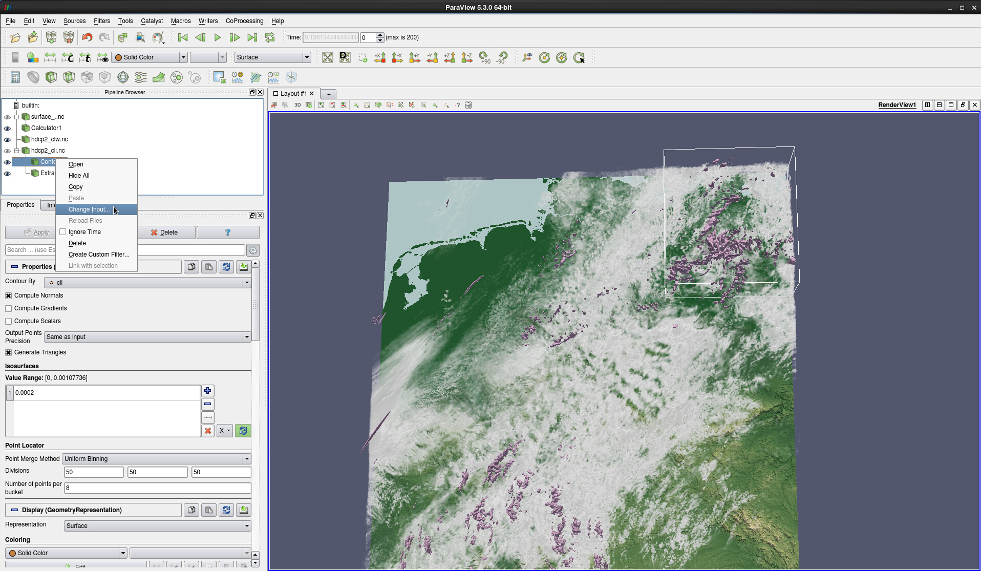
Figure 20: Change input of Contour
Looking at the Pipeline Browser, you will notice that both the Contour1 and the ExtractSubset1 module depend on hdcp2_cli.nc. To draw the isosurface for the subset only, you need to change the data input stream for the Contour module:
Right-click on the Contour1 module -> Change Input…
In the Change Input dialogue, select ExtractSubset1 -> OK
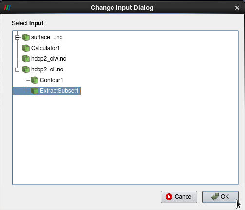
Figure 21: Change input of Contour1 to ExtractSubset1
The result is shown in Fig. 22.
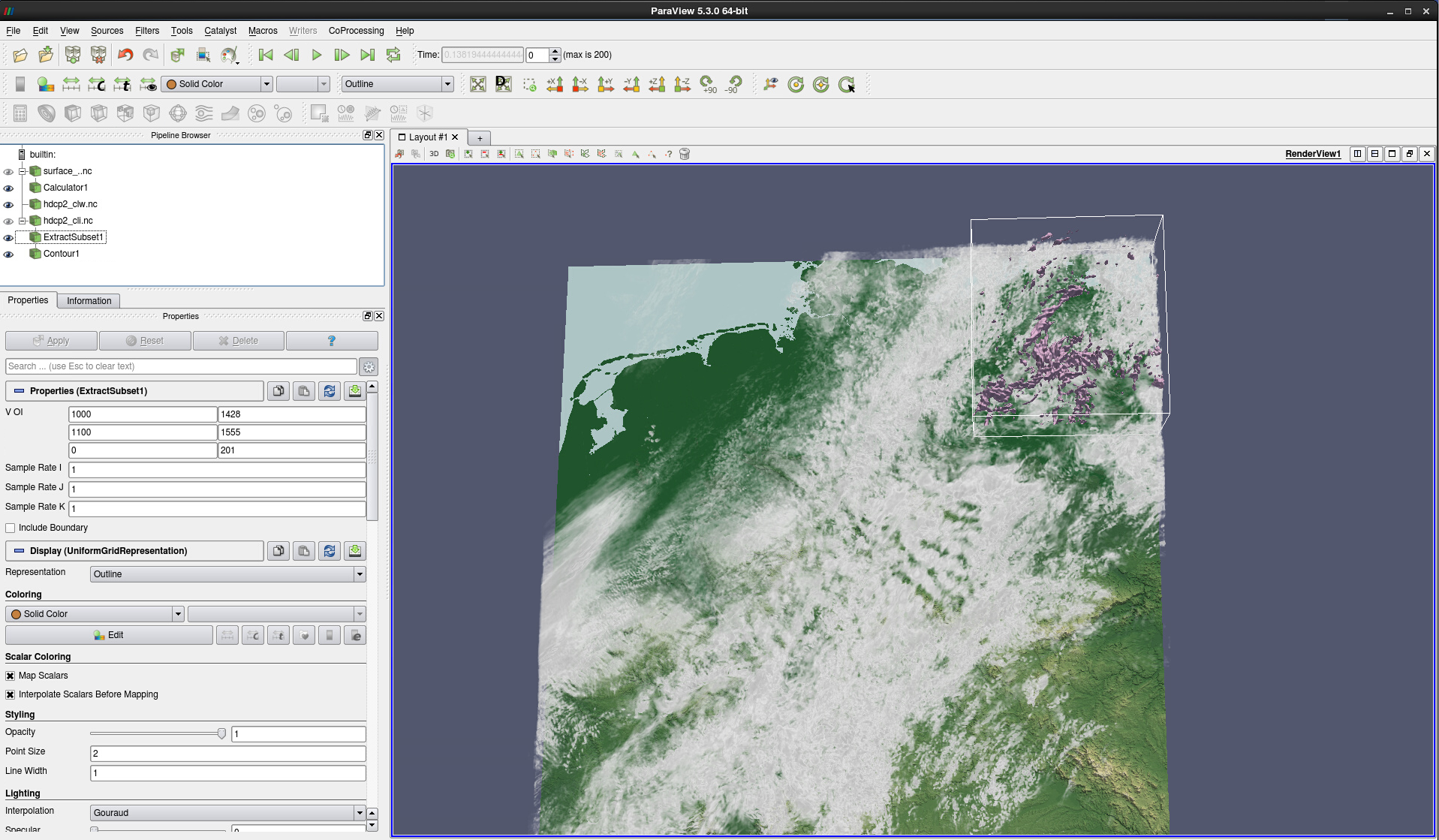
Figure 22: Contour1 applied to ExtractSubset1. The isosurface is drawn in the VOI box only.
Next, we are going to zoom in on the subset region and create a vertical cross-section of the cloud ice data by using a Slice filter.
Select the ExtractSubset1 module and click on the Slice button in the filters toolbar (see Fig. 23).
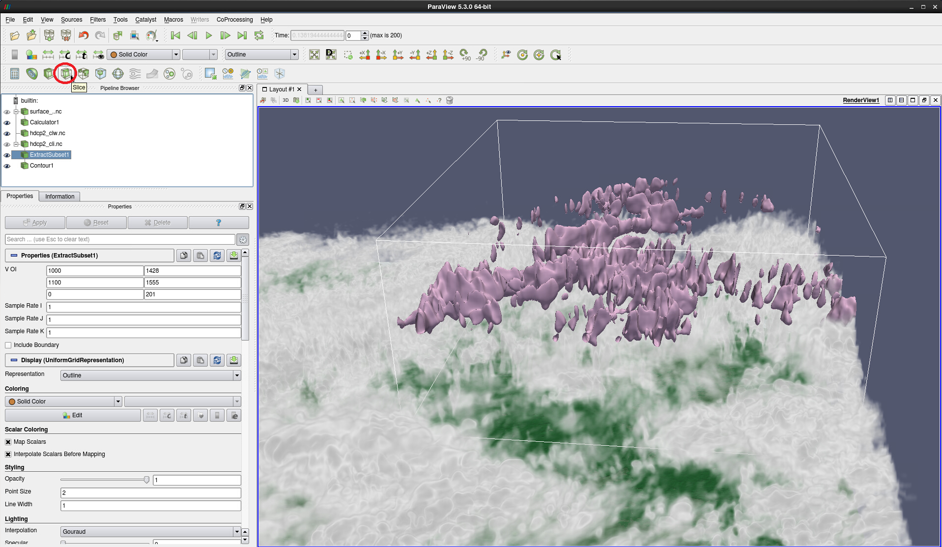
Figure 23: Close-up view of subset cli isosurface with Slice button highlighted
With Slice Type: Plane selected and Show Plane checked, the white slicing plane is displayed with a red rim and white handles. Use the mouse pointer to hover near the slice; theslice turns green and the handles turn red when they are active. You can grab the ends of the handle or the ball in the middle while pressing left mouse button, and thus tilt and move the slicing plane, or you can change the position of the handle itself relative to the slice. Explore the possibilities yourself; Note how the values in the input fields of the Plane Parameters change as you modify the slicing plane. To continue with the exercise we suggest that you use resize the ‘slicing box’ so that it approximately matches the size of the ExtractSubset1 box.
Next:
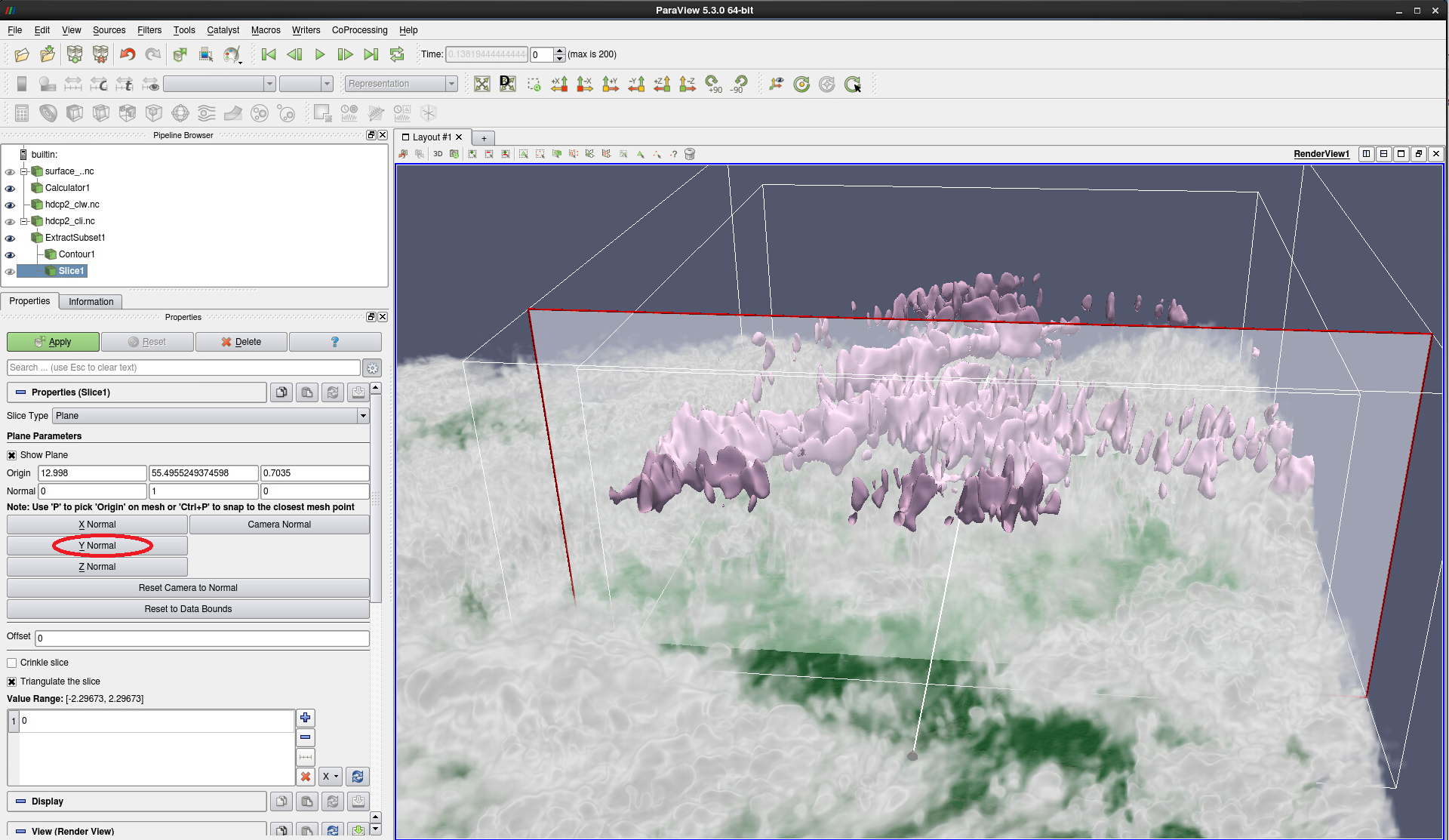
Figure 24: Properties of Slice filter before apply
Click on the Y Normal button in the Slice1 properties (see Fig. 24).
Move the slicing plane to the southern end of the box until it hardly intersects the edge of the pink cli isosurface.
Hit Apply
Compare your screen with Fig. 25.
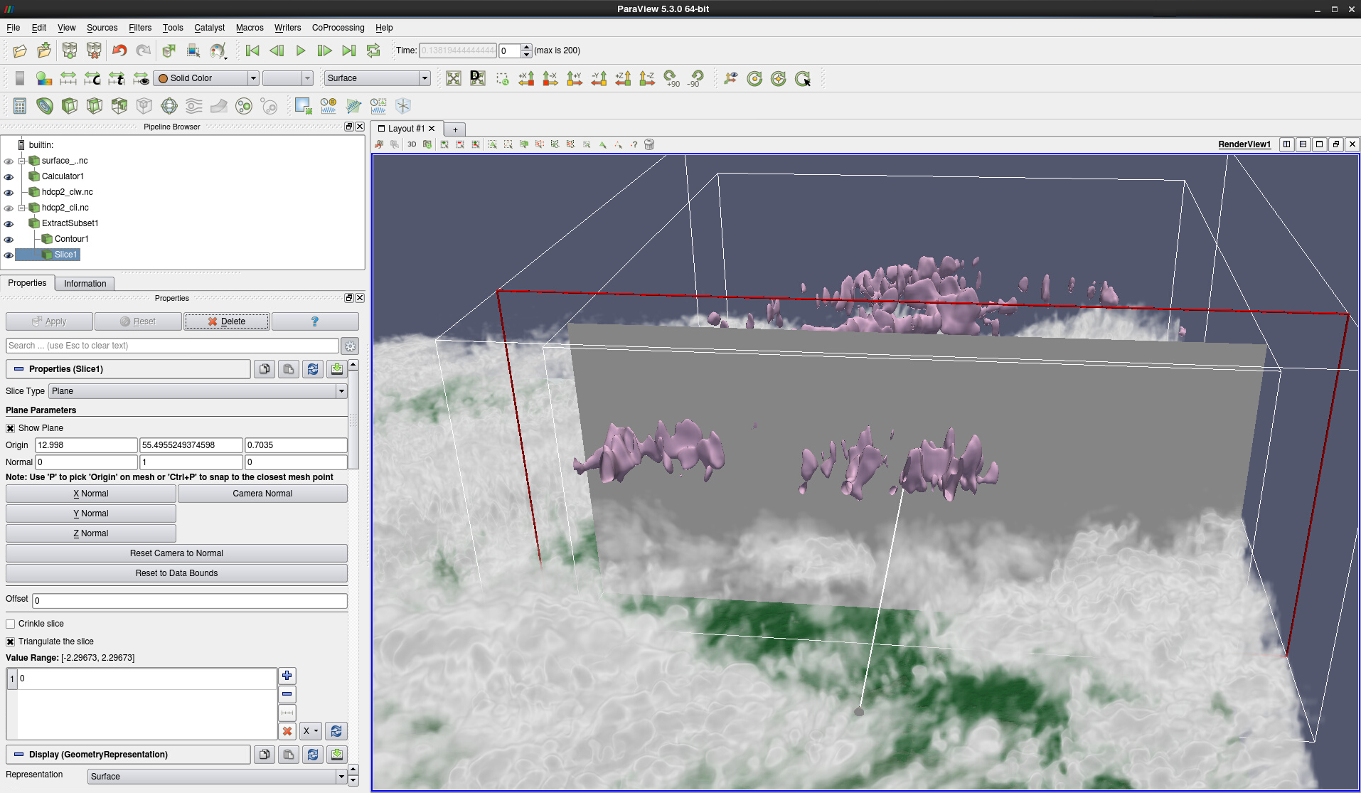
Figure 25: Slice with Y Normal applied, showing a Surface of Solid Color
Uncheck Show Plane
Change Solid Color to cli
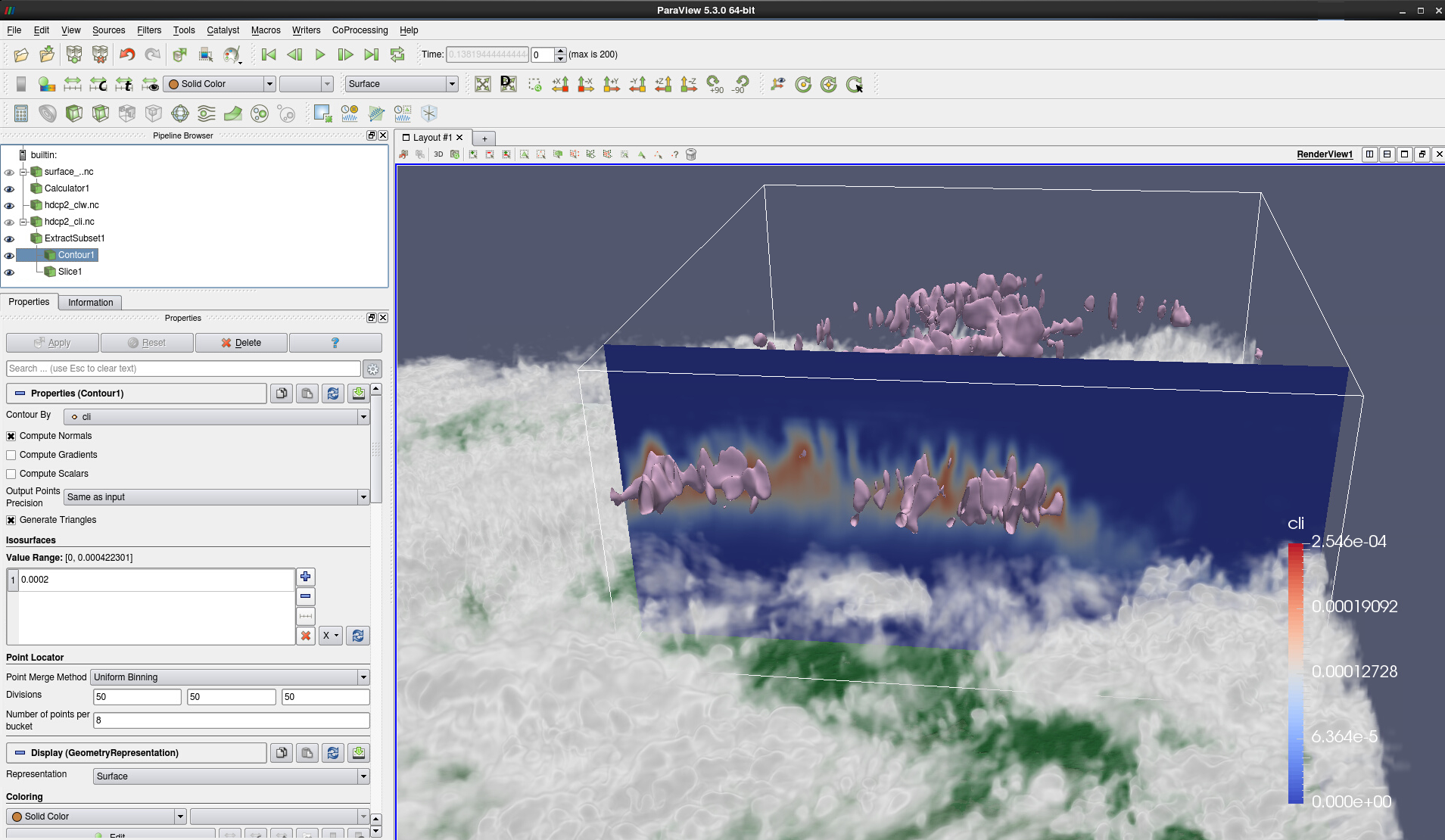 Figure 26: Slice with Y Normal applied and colored by cli
In following, we will generate isocontours for the current slice position, assign a different colormap, switch off the volume rendering of clw and decrease the opacity of the pink cli isosurface. The result is depicted in Fig. 28.
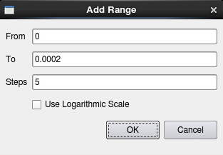
Figure 27: Add range of 5 contour values from 0 to 0.0002. See Fig. 28 for the result.
With the Slice module selected, click on the Contour filter in the toolbar
In the new Contour module, make sure that it says Contour by cli
Check Compute Scalars – only then can you color the isocontours by the variable they were created from (here: cli)
In the Isosurfaces section of the properties: remove the existing entry by selecting it and clicking on remove entry (red x button)
Click on add a range of values (button with the ruler symbol)
From 0 - To 0.0002 - Steps 5 -> OK (see Fig. 27)
Click Apply
In the Coloring section, change from Solid Color to cli
Change the coloring by Edit Color Map and / or by Choose preset (see above)
Optional: In the Styling section, you may change the LineWidth to a value of 2
Switch off the volume rendering of clw by clicking on the eye symbol next to hdcp2_clw.nc
In the Styling section of the isosurface Contour1, decrease the opacity slider, e.g. to a level of 0.55.
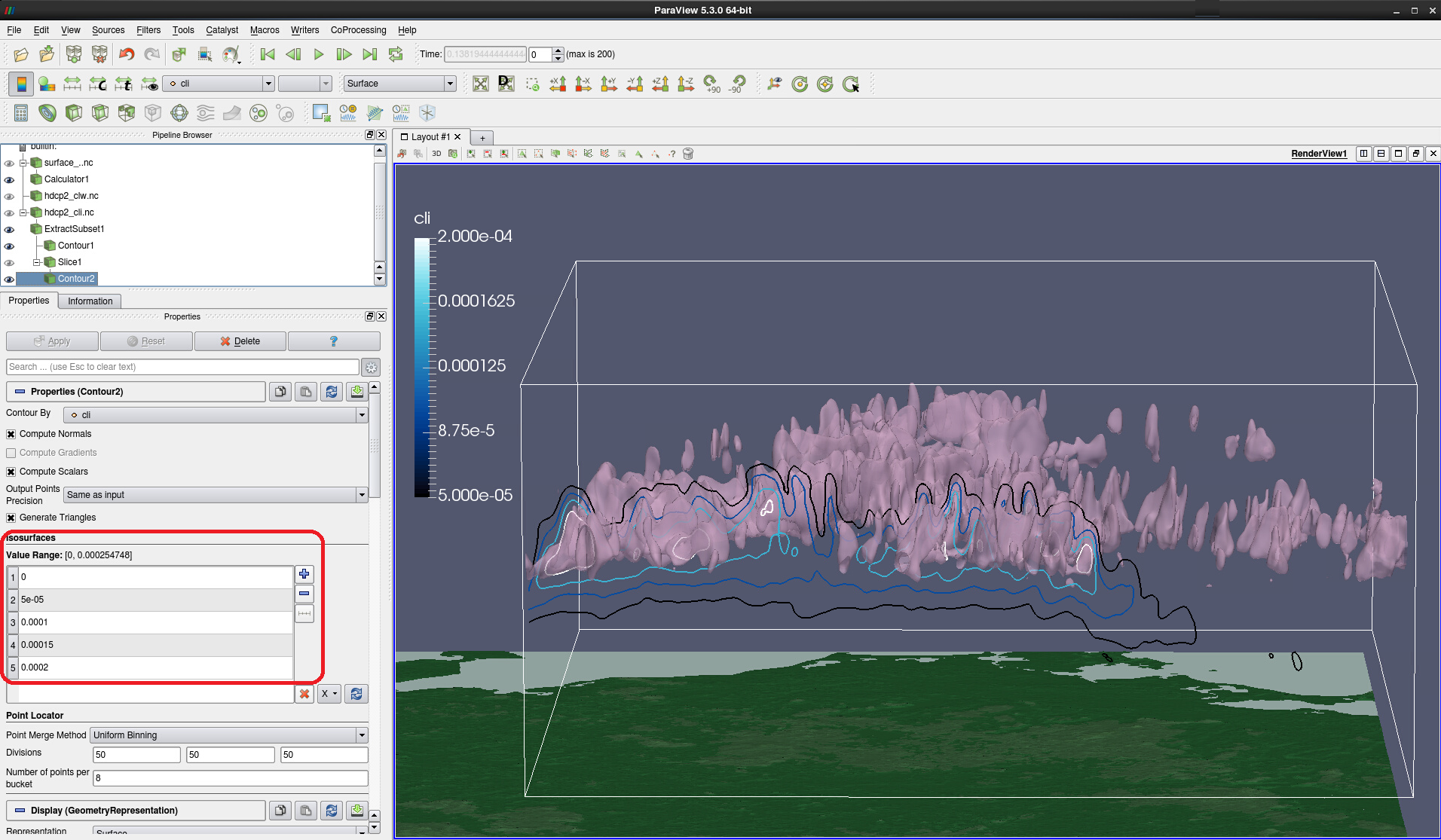
Figure 28: Isosurface and five discrete isocontours for cli
Don’t forget to save your project. If you like, continue with :ref:`export-animation`.