Using an earth texture as background

A great resource for freely available earth textures are the NASA Blue Marble images (credit: Reto Stöckli, NASA Earth Observatory) from the Visible Earth collection, which we will also use in this tutorial example.

Equidistant cylindrical representation

When working with an equidistant cylindrical representation of global netCDF data, you simply need to load one of these global earth images and make some adjustments. If a global 5400 x 2700 px Blue Marble texture including topography and bathymetry suits your needs, you can start your visualization project by loading the following state file on Mistral: /work/kv0653/ParaviewTutorial/earth.pvsm

If you would like to use an equidistant cylindrical representation with a different texture than the Blue Marble image in the above state file, you have two options. Either you load the PNG image file into ParaView and scale and transform it accordingly, or you texture-map the image to a plane. Below, we describe both of these options:

Option 1: Loading and transforming a PNG image as background

• Load the respective image file into ParaView

• uncheck Map Scalars in the Scalar Coloring section (see Advanced Properties)

• Adjust Position and Scaling in the Transforming section

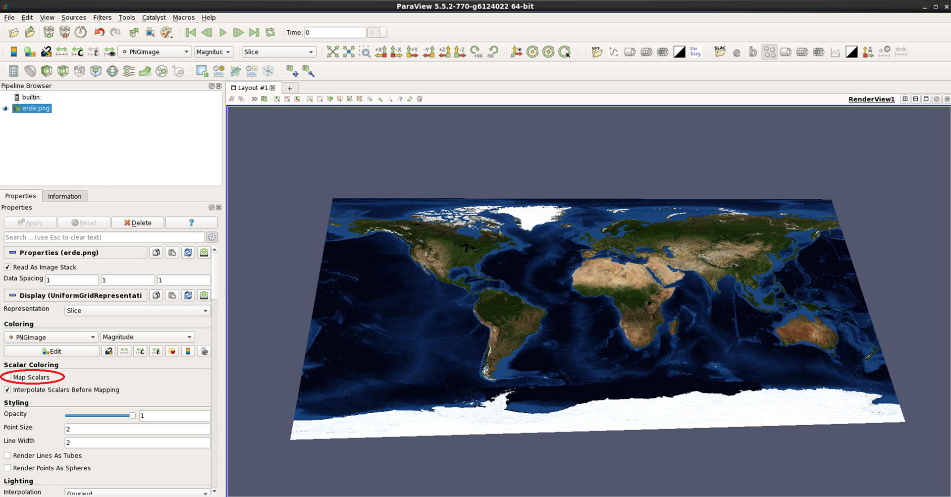
Figure 1: NASA Blue Marble Earth texture as background image for equidistant cylindrical representation

The following Transform values apply to images of size 5400 x 2700 px only and need to be adjusted for larger textures.

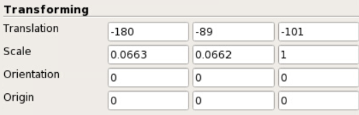Figure 2: Transform settings to prepare 5400 x 2700 px earth texture as background image for equidistant cylindrical projection

To check if your earth background is scaled and positioned correctly, we suggest loading a dataset that clearly shows the signature of oceans and continents, such as surface temperature t in ECHAMH_OM_A1B.nc, which is available in the ParaView tutorial folder on Mistral. Note that you may have to adjust the vertical scaling or position of the dataset.

Option 2: Texture-mapping to a plane

To create a plane of the proper size, we suggest that you first load the dataset for which you need a background image. This is optional, however, it helps ensure that the plane will be oriented and positioned correctly. Then:

• Select Sources -> Plane

• Fill out Origin, Point1 and Point2 in the Plane Properties using the Bounds of your dataset (see Information tab)

• Click Apply

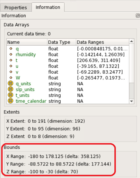
Figure 3: Dataset bounds to be used for defining a Plane

Size and position of dataset and plane will coincide if you enter the bounds of your dataset into the Plane properties as was done in figure 4. Note that the signs of the longitudes have been reversed. To be more exact, one could use -180, 180, -90, and 90 for x- and y-coordinates and 100 for the z-coordinate in the Plane properties. However, at least for the dataset that we used in this example, the texture background would look slightly larger than the data cube, and it would also interfere with the lowest data level. When working with a global dataset, we would therefore suggest using the data bounds in the Plane properties, because the difference in scaling will be negligible.

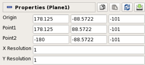
Figure 4: Setting the Plane properties according to the ECHAM dataset bounds

 The next steps will be:

• With Plane1 selected, add Filters -> Alphabetical -> Texture Map to Plane

• Click Appy

• In the Miscellaneous section of Texture Map to Plane, check Pickable Texture and load your desired earth image texture, such as erde.png from the tutorial folder

• In the Transform section, set the third, i.e. z-value of Translation to -101Compare your visualization result with the following figure:

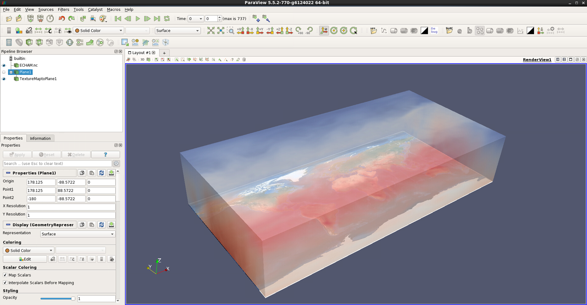
Figure 5: Data annotated with earth background image mapped to a plane

Spherical representation with texture mapping

To annotate a spherical representation of climate and earth system data, the earth background image needs to be loaded as a texture and “wrapped around” a sphere in ParaView. The steps, which we are going to cover in detail hereafter, are as follows:

• Prepare texture image or select one that has already been prepared

• Create a sphere source in ParaView

• Apply filter Texture Map to Sphere

• Select Pickable Texture in the Miscellaneous section of the properties

• Check proper positioning of the texture

Prepare image texture

In case you simply try to map the earth image texture from the previous section to a sphere in ParaView, you will notice that the result won’t look right. To solve the issue, you may use one of the following textures from the ParaView tutorial folder.

• erde_flipped2.png                                                                       (light blue ocean bathymetry)

• erde_flipped2_bw.png                                                                 (grayscale)

• erde_flipped2_bw2.png                                                               (grayscale)

• world.topo.200408.3x5400x2700_ParaView.png                        (topography only)

• world.topo.200408.3x21600x10800_ParaView.png                    (topography only, high resolution)

• world.topo.bathy.200408.3x5400x2700_ParaView.png               (topography & bathymetry)

• world.topo.bathy.200408.3x21600x10800_ParaView.png           (topography & bathymetry, high resolution)

However, if you would like to use a different one or if you are just curious, we suggest the following steps to prepare the image for spherical texture mapping in ParaView. Using an image editing software of your choice, you need to:

1. Flip the image vertically

2. Cut it in the middle and swap the lateral position of the two image parts

3. Use retouching to remove some artifacts at the bottom where the two image parts meet.

Before:

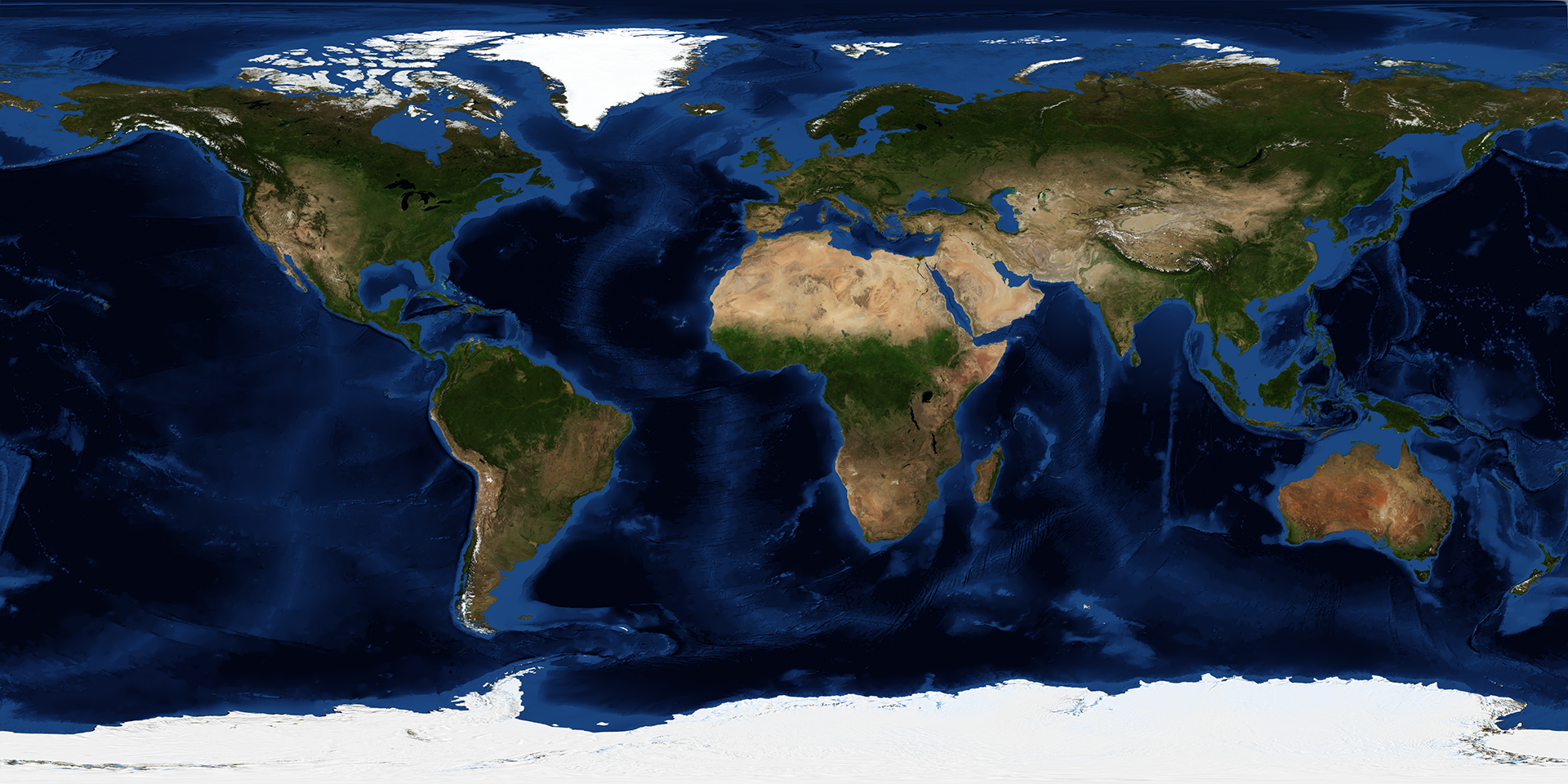
Figure 6: NASA Blue Marble earth texture showing topography and bathymetry

After:

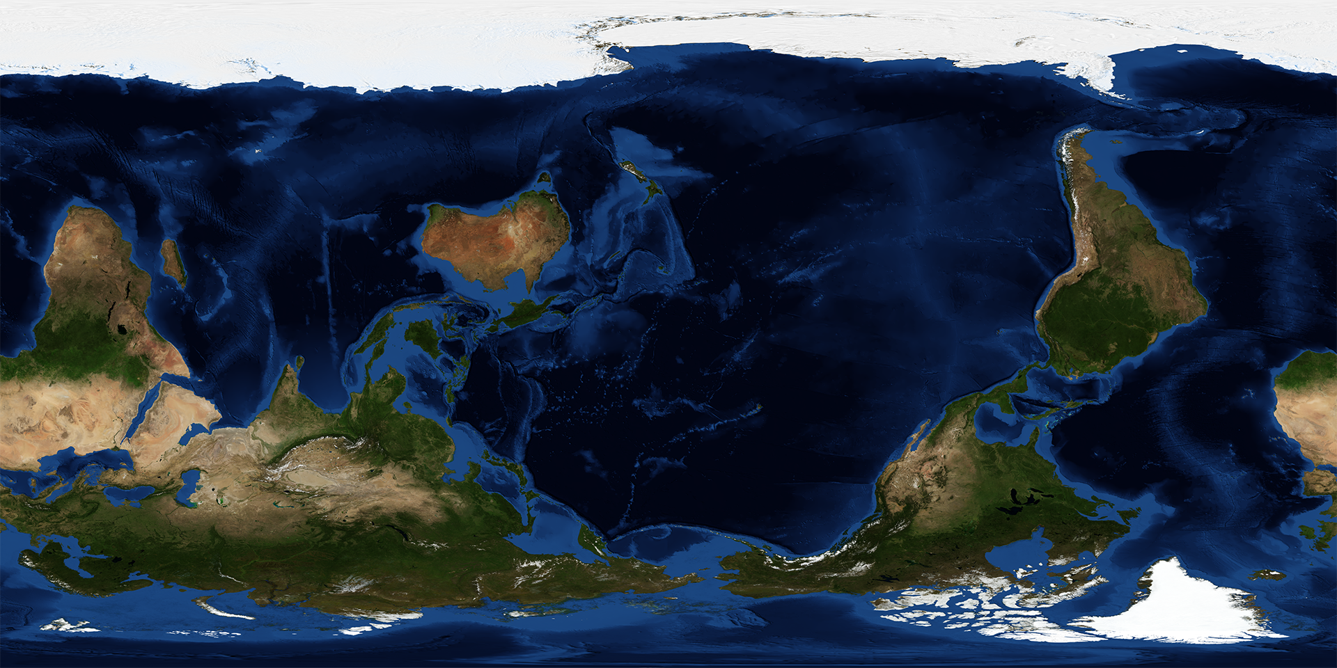
Figure 7: NASA Blue Marble earth texture prepared for texture mapping on a sphere

The Imagemagick commands for flipping, swapping and merging are:

convert -flip -crop 50%x100% filename.png converted.png
convert converted-1.png converted-0.png +append outfile.png

Don’t forget to remove the cropped image parts converted-0.png and converted-1.png afterwards.

Texture Mapping in ParaView

Start with an empty ParaView session by either opening ParaView or by clearing the Pipeline Browser via Edit ->  Reset Session.

Steps:

1. Sources -> Sphere

2. Set Radius to 1, Theta & Phi Resolution to 50 or 100 and Start Theta to 1e-5

3. Click Apply

4. Filters -> Alphabetical -> Texture Map to Sphere

5. Uncheck option Prevent Seam

6. Click Apply

7. In Property section Miscellaneous, check Pickable Texture

8. Change None to Load… and navigate to the image texture file, click OK

Compare with the following figure:

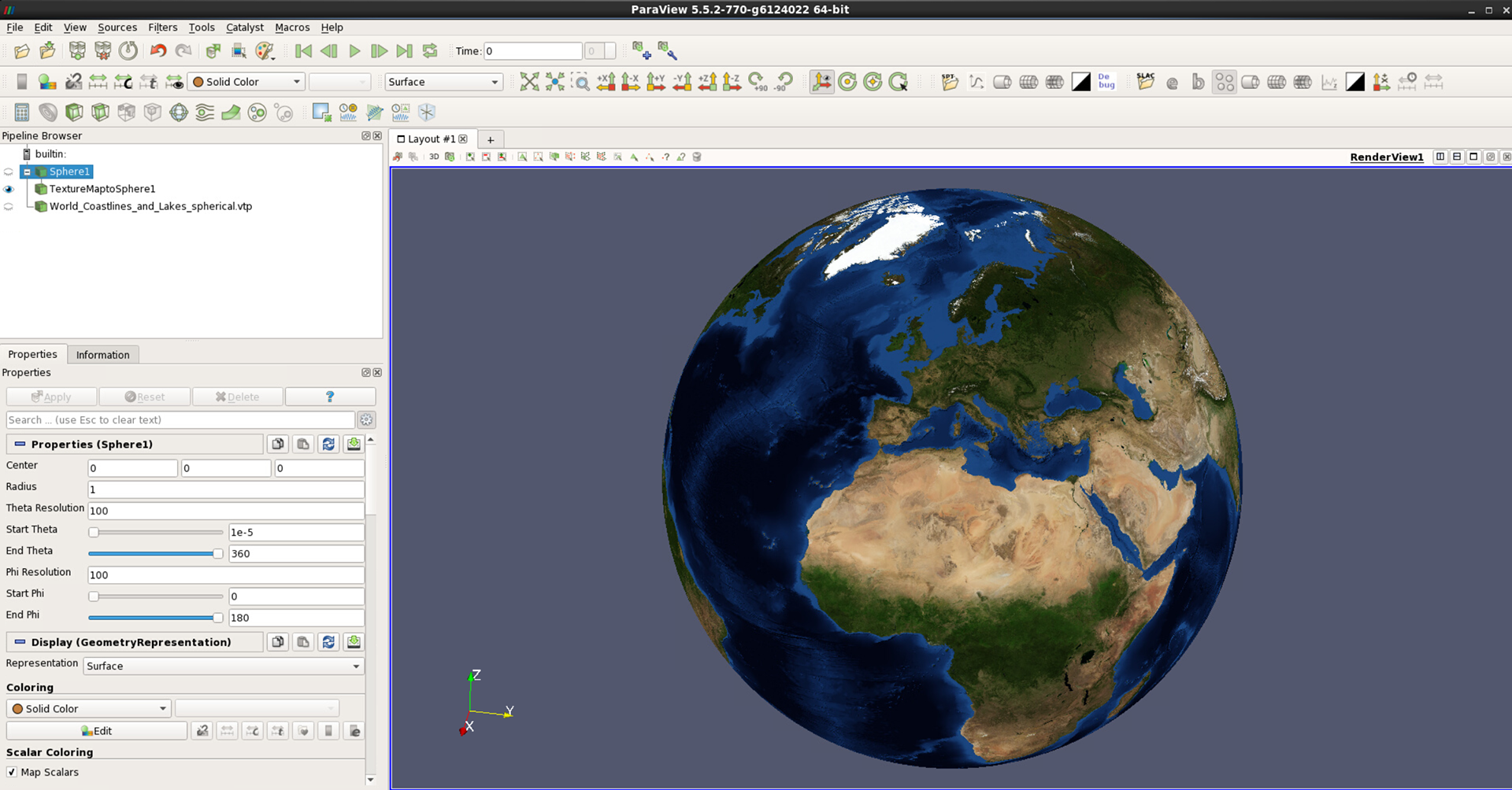
Figure 8: Earth texture mapped to sphere

To check the proper positioning of the texture we suggest loading a coastline dataset for spherical projections, such as: /work/kv0653/ERDE/World_Coastlines_and_Lakes_spherical.vtp.

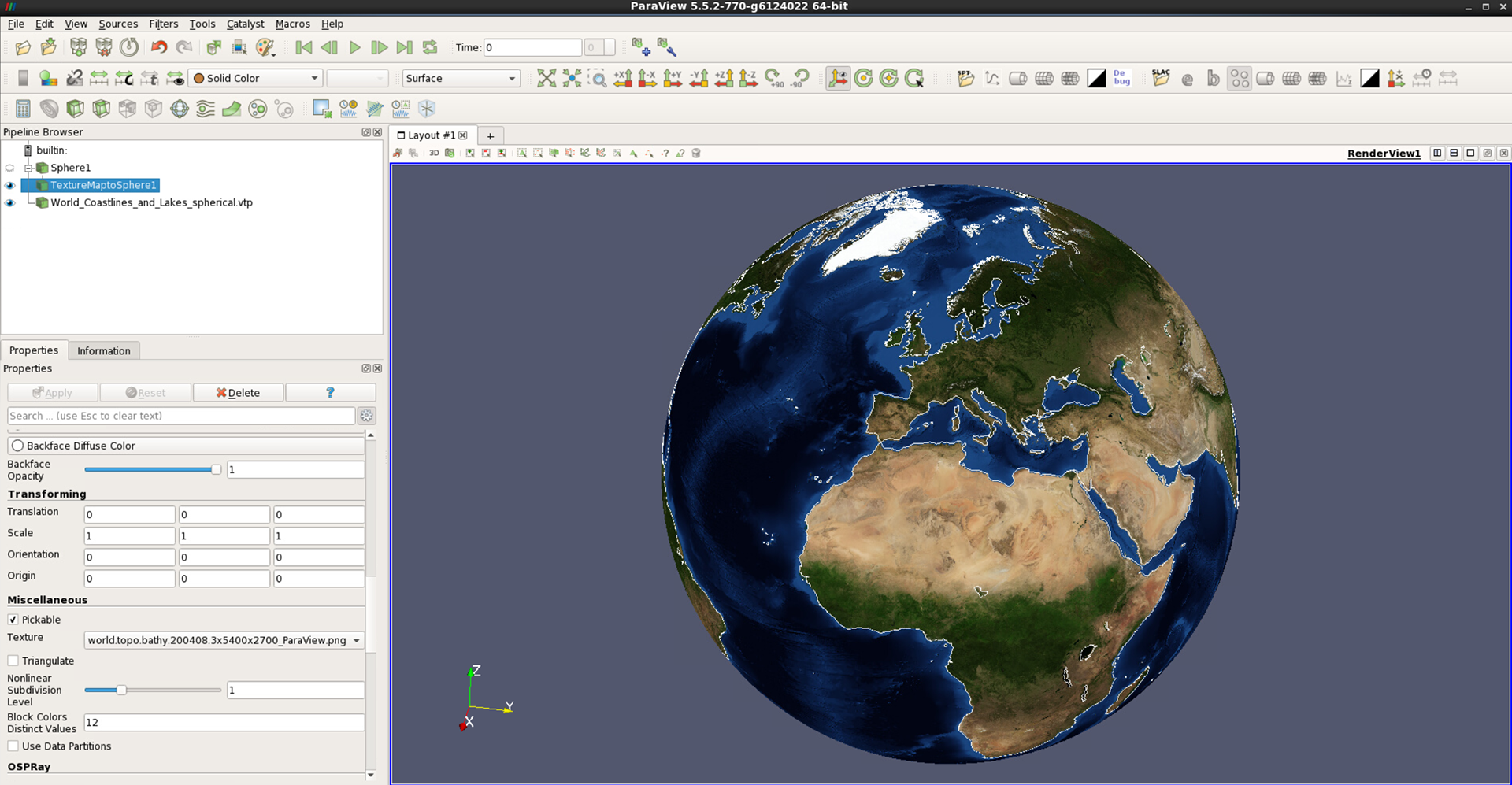
Figure 9: Earth texture mapped to sphere with coastlines

Combining  extrusion (exaggerated orography and bathymetry) and texture mapping

It is possible to extrude topography and bathymetry in addition to using an earth texture. For details on vertical exaggeration using the Calculator module, see here:

The visualization workflow is as follows:

1. Load high – resolution topography data (e.g. ETOPO1 data in netCDF format) with desired projection

2. If necessary, add filter Cell Data to Point Data

3. Add Texture Map to Plane or Texture Map to Sphere

4. Add a Calculator filter to perform extrusion as described here – be sure to check & adjust the name of the height variable (altitude, z, etc.) in the formula

5. Set Pickable Texture in the Miscellaneous section of the Calculator module

You may want to adjust the lighting of the scene via View -> Light Inspector.

Equidistant cylindrical projection

The following figure shows a corresponding screenshot of the equidistant cylindrical projection with the representation set to Surface.

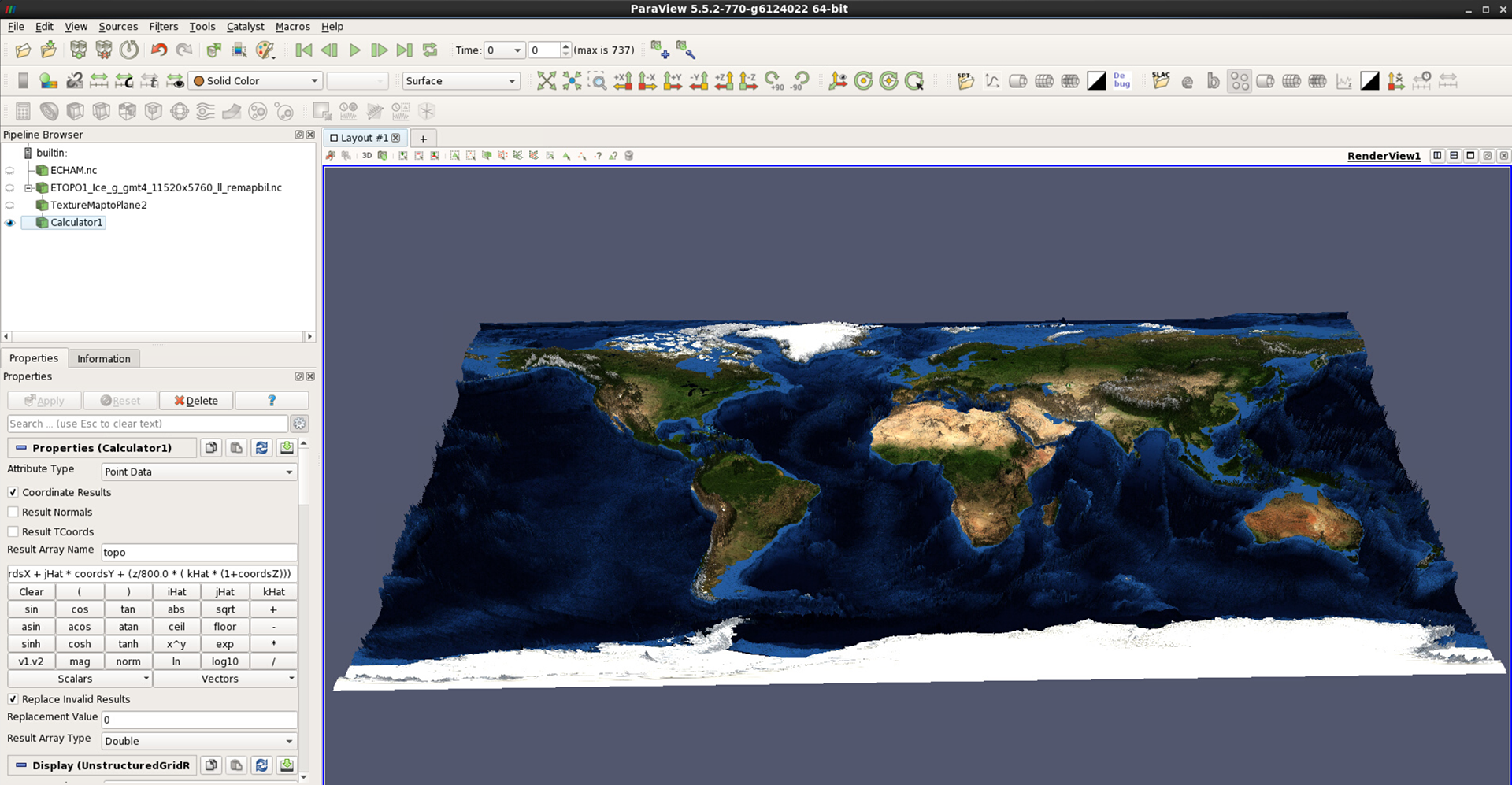
Figure 10: Earth texture mapped to equidistant cylindrical representation of exaggerated topography and bathymetry

Spherical projection

With a spherical projection, the extruded and texture-mapped surface looks as follows:

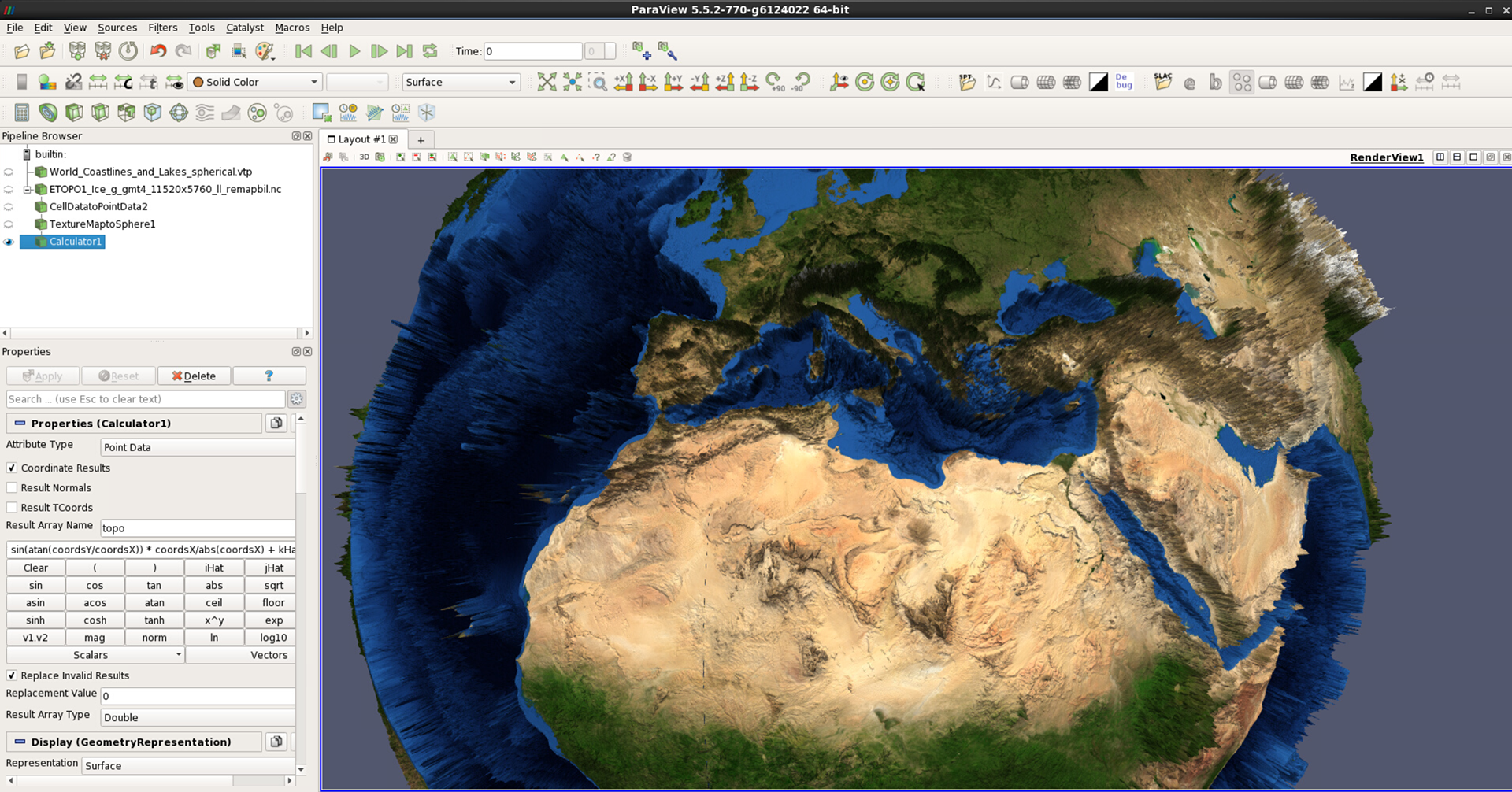
Figure 11: Earth with texture map and exaggerated topography and bathymetry represented as Surface

The topographic and bathymetric features stand out nicely. However, a seam is clearly visible over the Sahara desert in Northern Africa. One makeshift solution is changing the representation from Surface to Points, as was done in figure 11. However, this, too, comes at a cost. Topographic and bathymetric features look significantly less crisp and shaded, and at steep slopes / seamounts in the ocean the point representation becomes obvious.

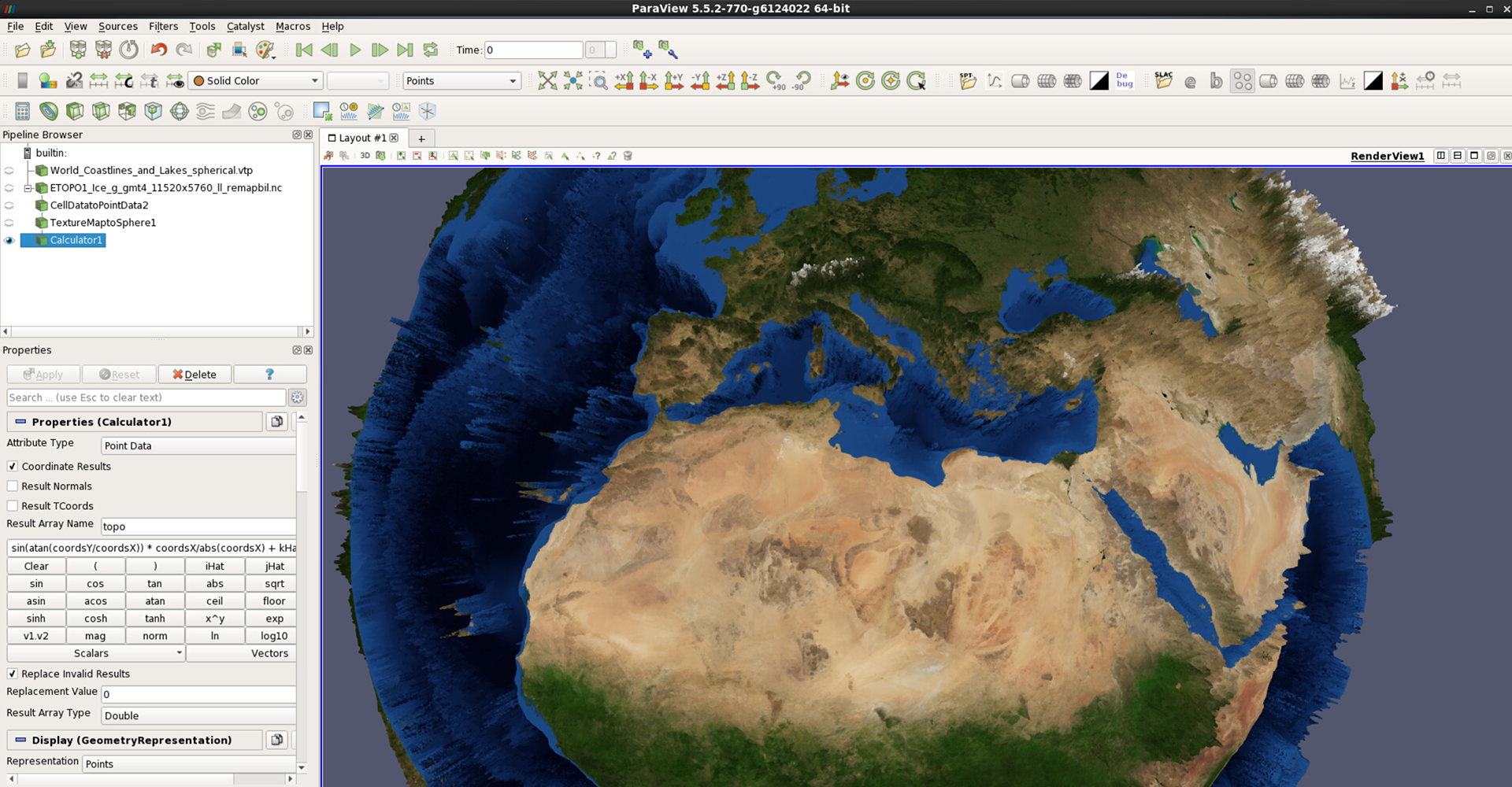
Figure 12: Earth with texture map and exaggerated topography and bathymetry represented as Points

When done, remember to save your ParaView visualization project as a state file.