Volume rendering of (NARVAL II) ICON data#
Area: HD(CP)² NARVAL II study area – Tropical Atlantic (DOM01)
Load your previously created map background
File -> Load state… -> e.g. NARVALII_background.pvsm (or whichever state file name you used )
Check that the path to Dom1_Surface.vtu is correct
Press OK
In a next step we are going to load the data set NARVALII_DOM01_small.nc, which is defined on the original ICON grid.
Load the data set
File -> Open… -> NARVALII_DOM01_small_qv.nc
Press OK
Select CDI netCDF Reader (ICON) – see Fig. 1
Press OK – see Fig. 2
Check cell variable qv, Project Lat/Lon and Show 3D Surface
Set the 3D Surface Thickness to 500
Press Apply
![]()
Figure 1: Select CDI netCDF Reader (ICON)
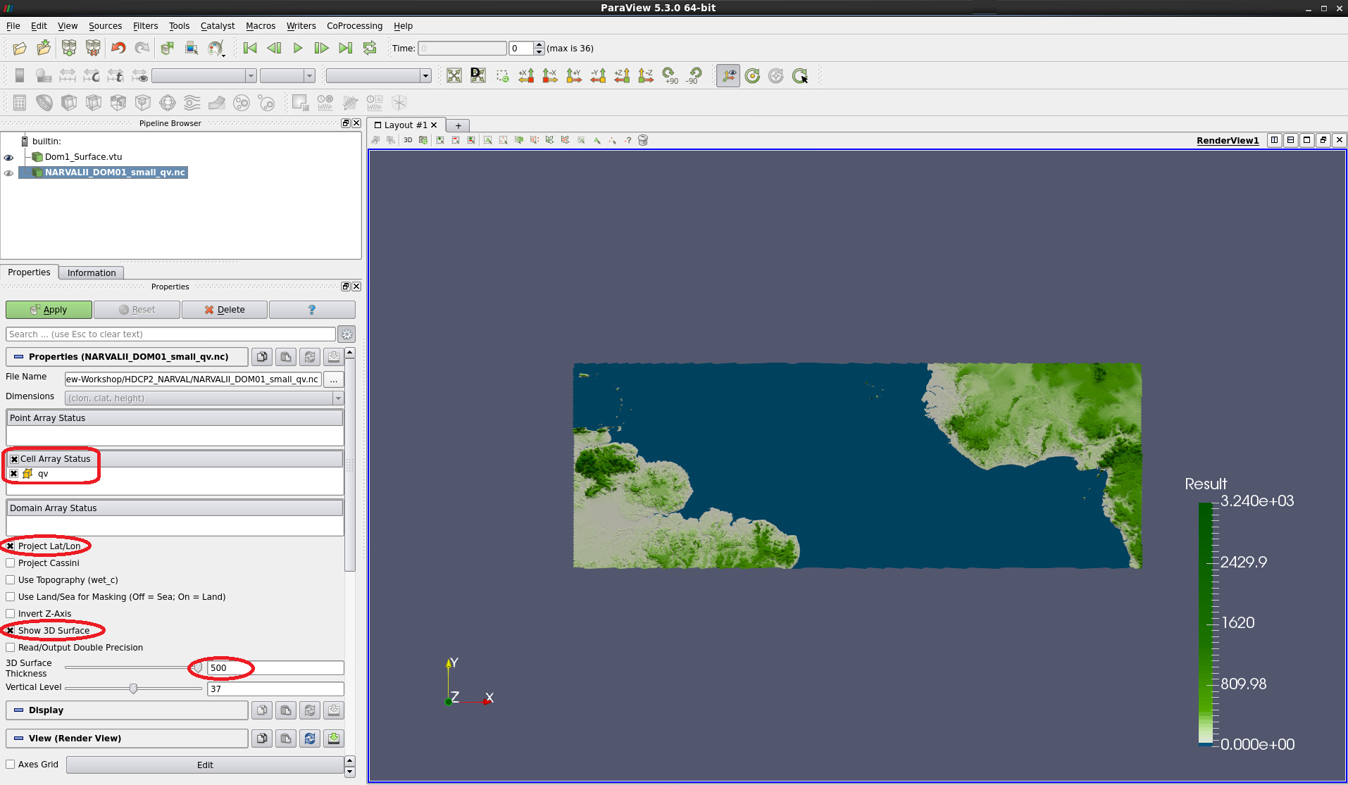
Figure 2: Prior to applying the data,check cell variable qv,Project Lat/Lon,Show 3D Surfaceand set3D Surface Thicknessto500
Tilting the visualization in the viewer one notices that most of the 3D surface is below the map background – compare Fig. 3.
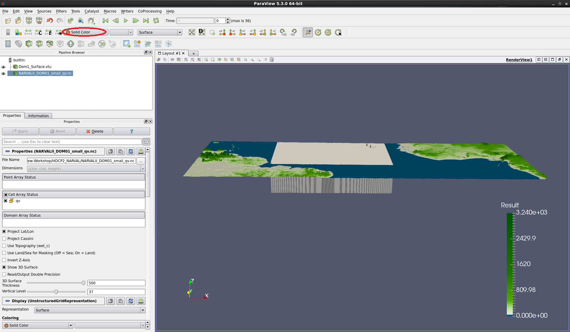
Figure 3: Data as 3D Surface applied. Most of the surface block lies below the background map
In the Properties of Dom1_Surface.vtu:
Scroll down to the Transforming section
Enter -8 into the rightmost box behind Translation
With NARVALII_DOM01_small_qv.nc selected, change from Solid Color to qv
Switch off the background colormap legend by clicking on the colormap symbol (Toggle Color Legend Visibility) in the toolbar. Compare with Fig. 4.
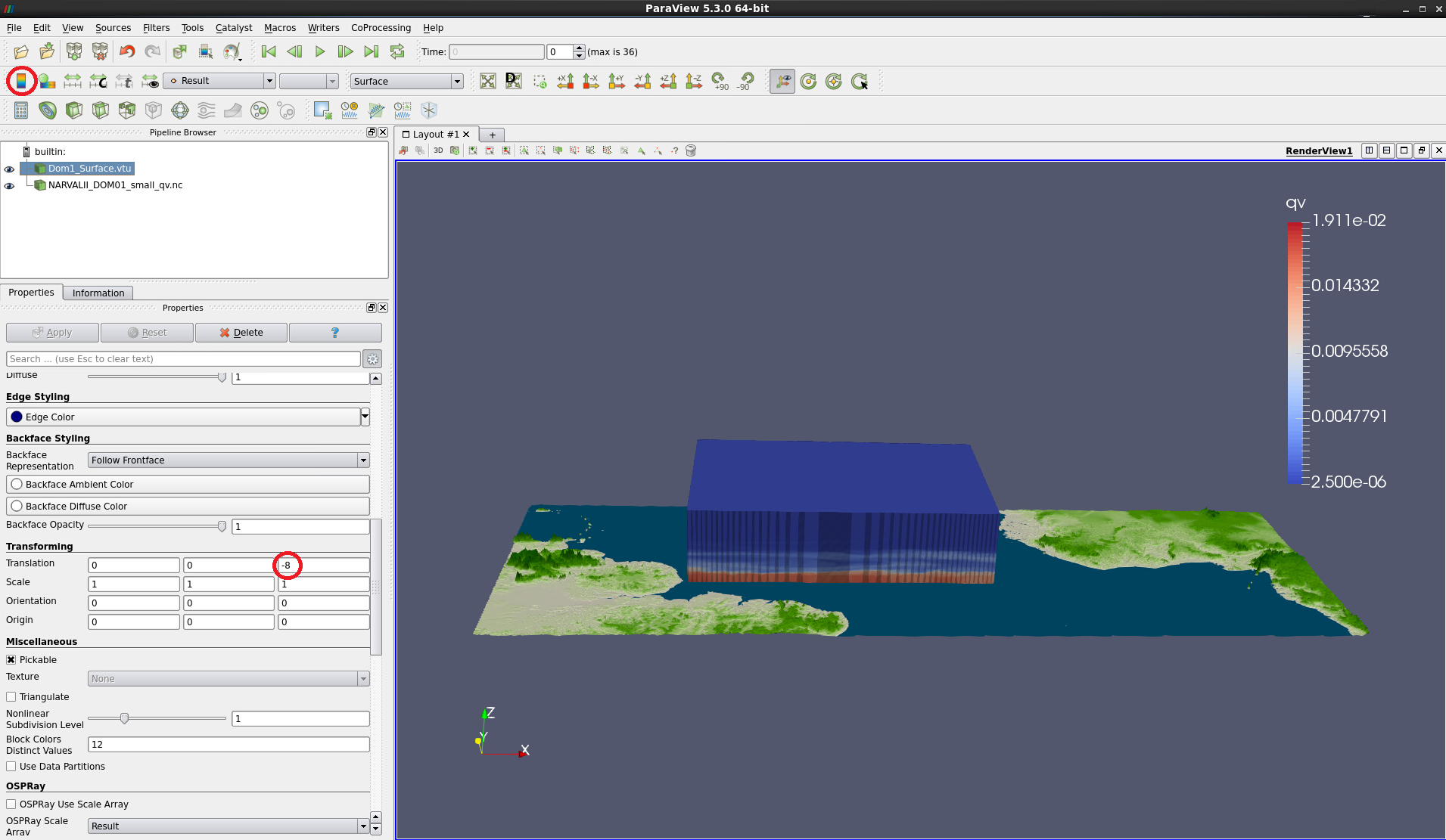
Figure 4: 3D surface colored by qv. Background map has been shifted vertically by -8.
To get an idea of the interior structure of the 3D specific humidity data volume we have at least three options. We can slice through the data or clip away a portion or we can use the volume rendering technique, where every voxel is assigned RGB color and opacity values. Trying to do volume rendering on a 12 GB data set such as NARVALII_DOM01_small_qv.nc is extremely costly and ParaView would likely freeze if you simply changed the representation from Surface to Volume. – Therefore please don’t. Instead we are going to resample the data on the fly to a regular grid and additionally use a threshold filter to exclude low data values.
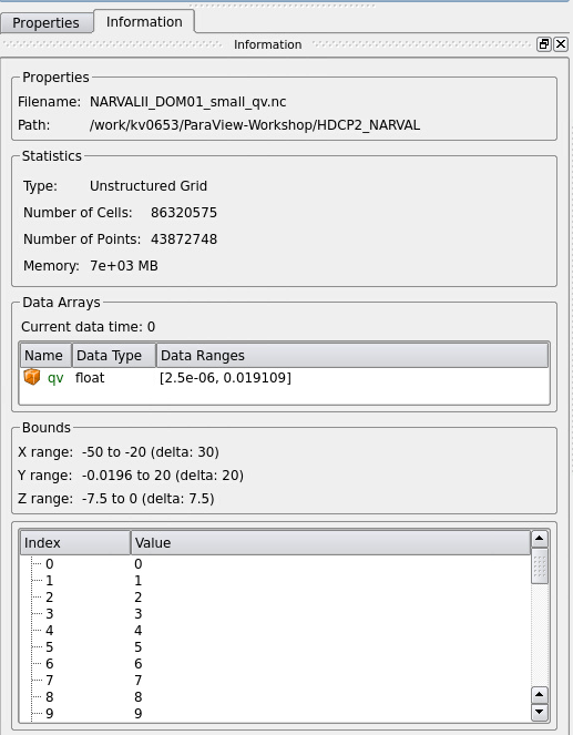
Figure 5: Information on data set NARVALII_DOM01_small_qv.nc
With the humidity data selected, go to Filters -> Alphabetical -> Resample to Image (see Fig. 6)
Figure 6: Selecting the Resample to Image filter
In the Properties of Resample to Image1:
Check Use Input Bounds
In the Sampling Dimensions fields try 1100 - 900 - 75 or 550 - 450 - 75 (see Fig. 7)
Click Apply
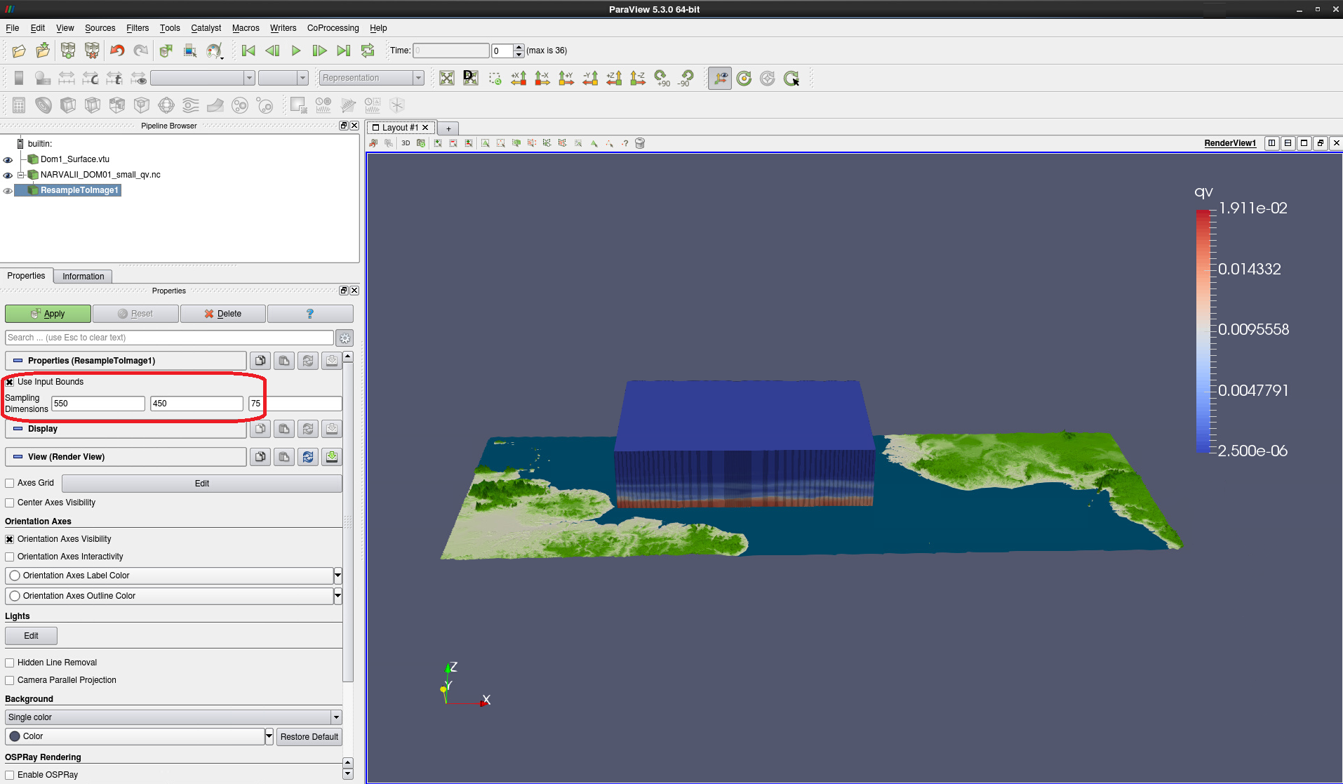
Figure 7: Settings for data resampling to a regular grid. All 75 height levels are maintained
Change the appearance of Resample to Image1 from Outline to Volume (see Fig. 8)
In the toolbar, click on Rescale to data range, the ruler symbol to the right of the colorbar symbols.
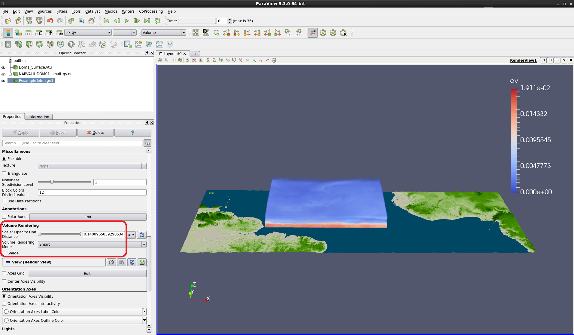
Figure 8: Volume rendering of data resampled to a regular 550 x 450 x 75 grid
Have a look at the Information tab of the Resample to Image output (see Fig. 9). The memory in use for the current time step is only 130 MB and much smaller than the 7 GB for the unstructured input data set (see Fig. 5).
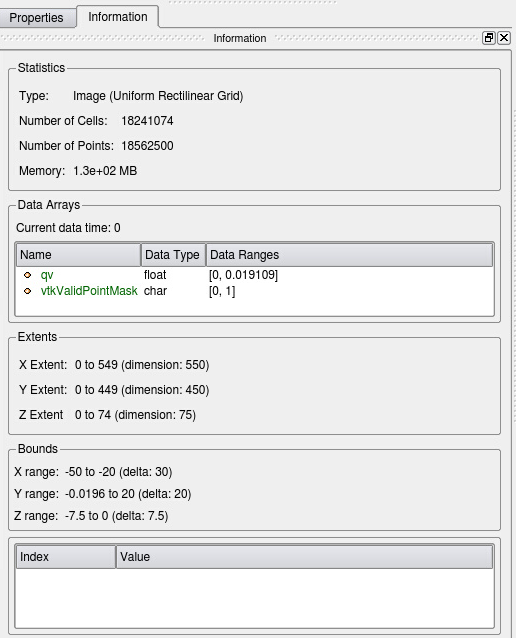
Figure 9: Information on output of Resample to Image. Memory usage is 130 MB
Play with the Scalar Opacity Unit Distance in the Volume Rendering section of ResampleToImage1 to see how the volume visualization changes (see Fig. 10).
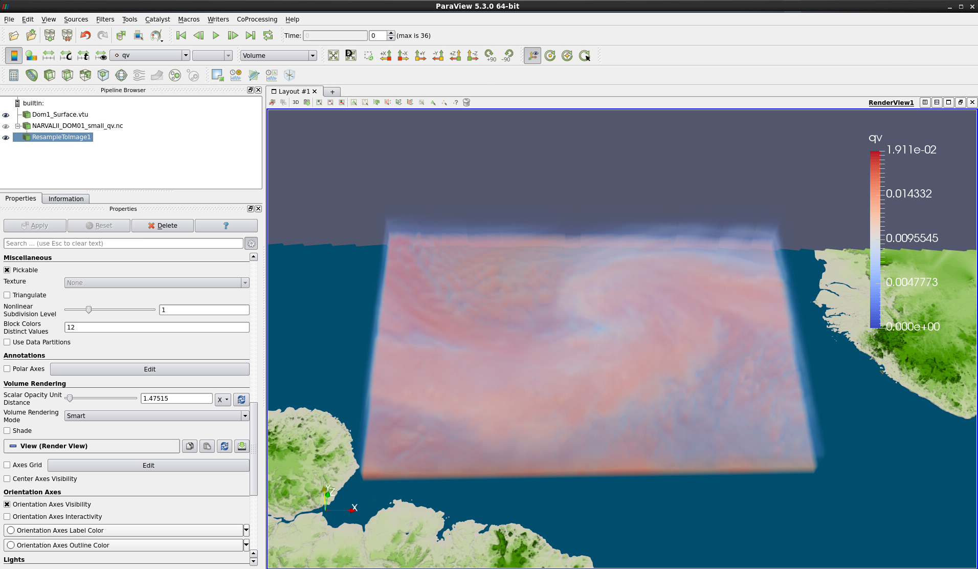
Figure 10: More transparent volume rendering of resampled data
Note
The resampled data can be stored on disk as a file series of VTK Image Data (.vti), a native ParaView format, for later use. Please don’t do this now, as the process would take time and disk space, but the procedure would be to click on File -> Save Data…, to navigate to the folder of your choice, set a file name and choose the format VTK Image data (see Fig. 11). The settings for the Writer would be Write all time steps as file-series and Data Mode Binary (see Fig. 12).
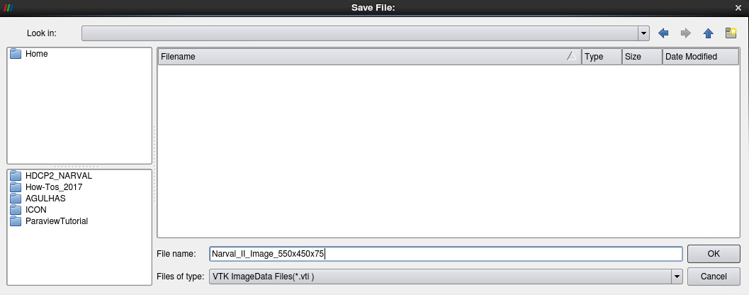
Figure 11: Saving VTK Image Data (i.e. regular data)
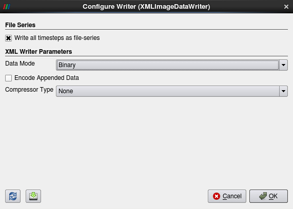
Figure 12: Configure Writer for saving VTK Image Data files to disk.
This data export would create as many files as there are time steps in the data. In the HDCP2_NARVAL/ workshop folder there are some .vti files that you could try to load in another ParaView session if you are interested.
Let us now apply a Threshold filter to exclude low data values:
Apply the Threshold filter :
With Resample to Image1 selected, click on the Threshold filter in the toolbar (see Fig. 10)
Change the sliders of Minimum and Maximum to values of your choice
Click Apply
Change the representation to Volume
This will take some time, especially as the output of the Threshold filter is unstructured again. – Compare Fig. 13. This data set takes up 900 MB of memory and interacting with the volume representation is somewhat tedious, because the default mapper is Projected tetra. However, one can select a different mapper and thus use Resample to Image on the fly:
Display Threshold filter output using volume rendering:
In the Threshold1 Properties, scroll down to the Volume Rendering section
Select Mapper Resample to Image
Enter sampling dimensions as before, e.g. 550 – 450 – 75
If you like, adjust the Scalar Opacity Unit Distance
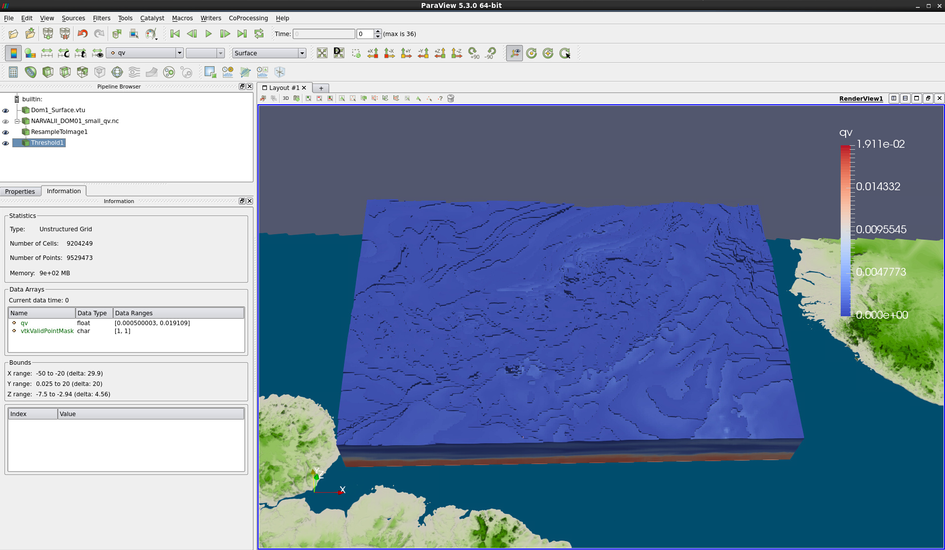
Figure 13: Threshold filter output as Surface representation and Information tab
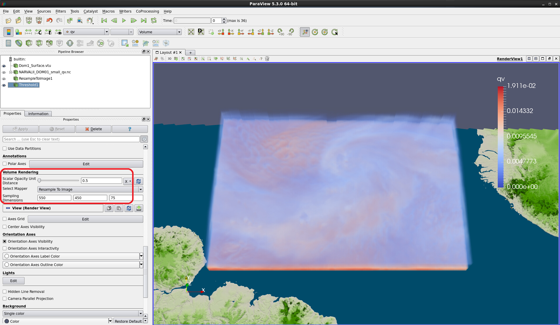
Figure 14: Volume rendering with minimum threshold of 0.0005.
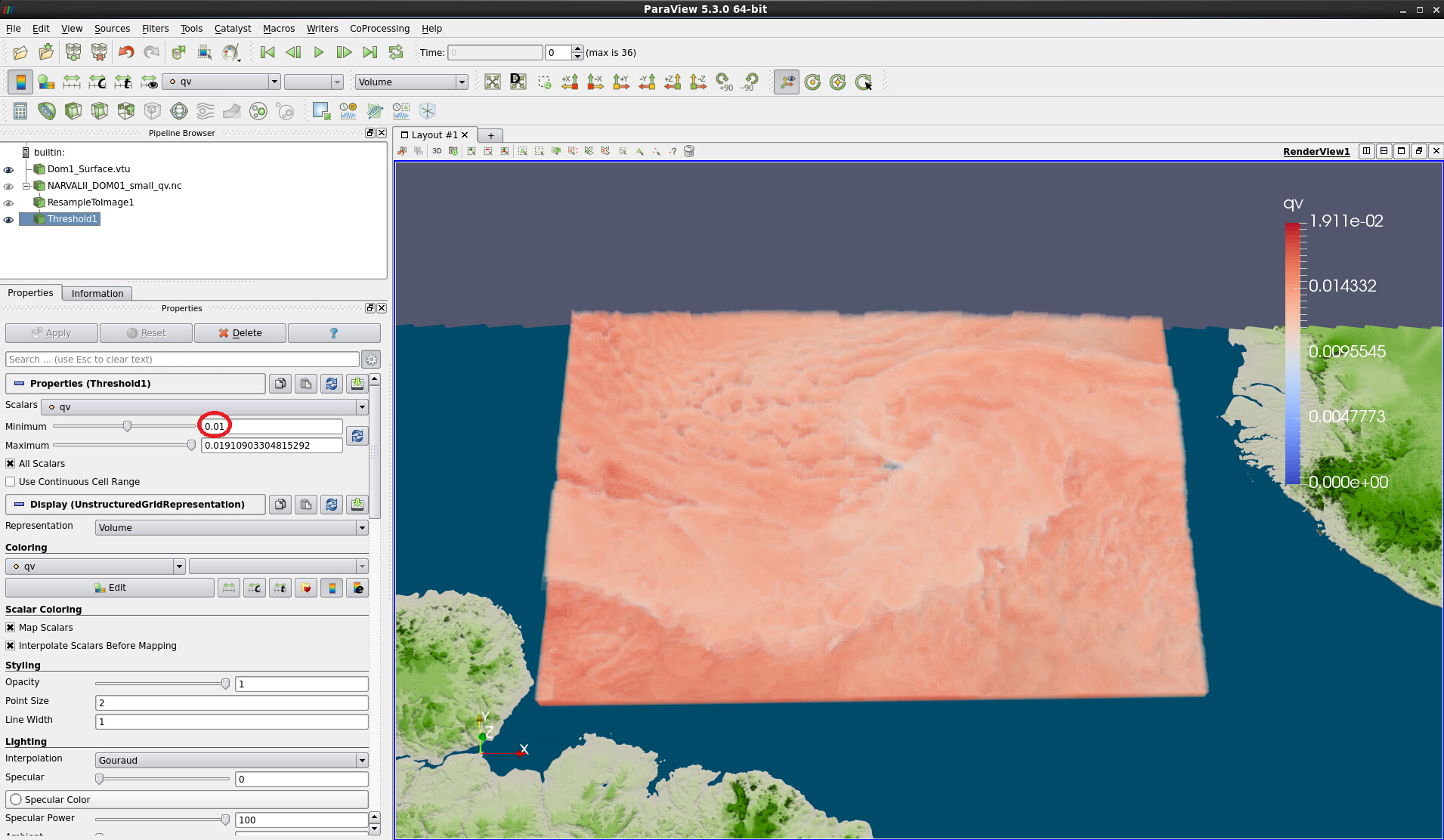
Figure 15: Volume rendering with minimum threshold of 0.01.
Finally, we suggest that you change the colormap for a more realistic rendering of the specific humidity using, e.g., color_qv.json (see Figs. 16 & 17). As this colormap has very low opacity values, you will need to change the Scale Opacity Unity Distance once more.
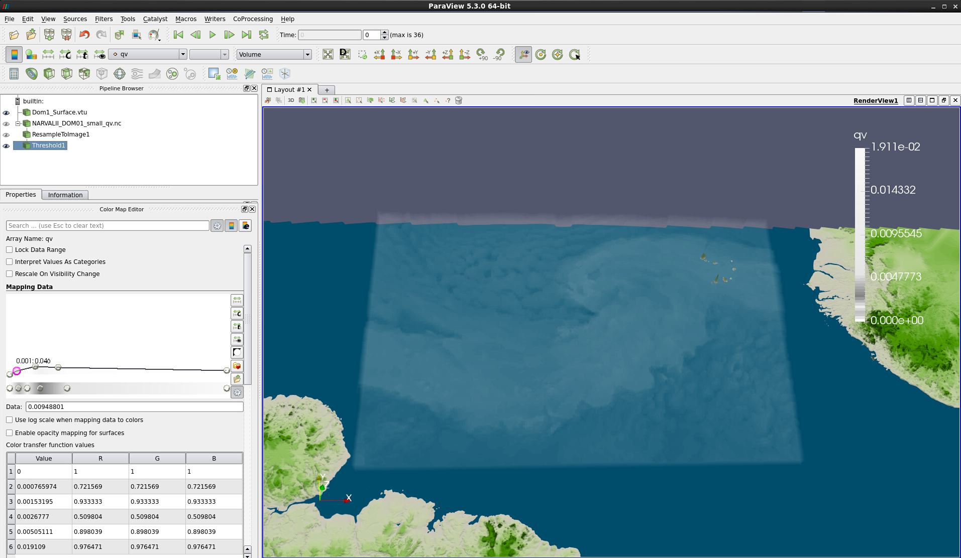
Figure 16: Volume rendering with the same threshold and colormap color_qv.json applied.
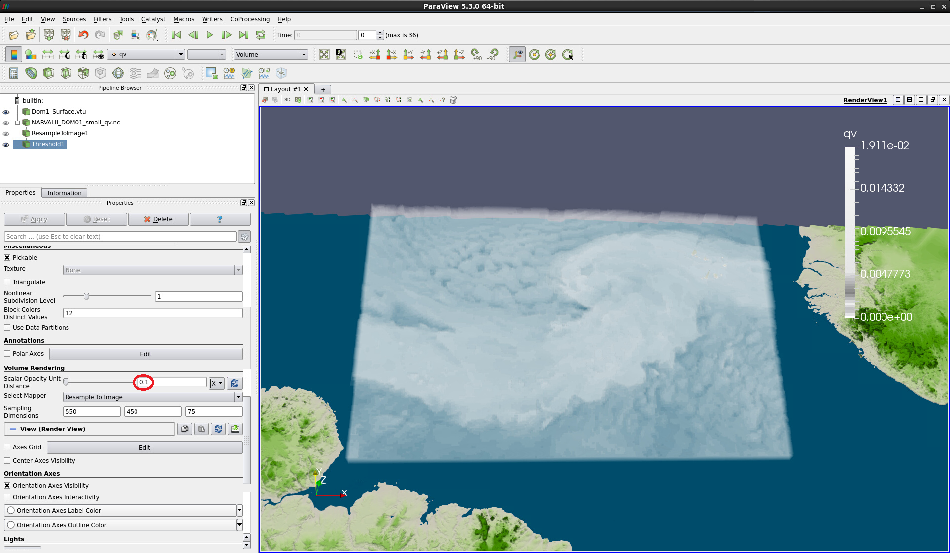
Figure 17: Same as Fig. 16, but with Scale Opacity Unity Distance adjusted
Note
If you think that the volume rendering representation looks too “flat”, you can always change the vertical scaling for individual modules in the Transforming section. Alternatively, you can increase the 3D Surface Thickness in the initial data module NARVALII_DOM01_small_qv.nc However, you will have to adjust the vertical position of the map background accordingly.