Streamline seeding in vector data

Area: HD(CP)² NARVAL II study area – Tropical Atlantic (DOM01)

Data directory: /work/kv0653/ParaView-Workshop/HDCP2_NARVAL/

Data file: NARVALII_DOM01_small.nc

Steps:

1. Load your previously created map background

• File -> Load state… -> e.g. NARVALII_background.pvsm (or whichever state file name you used )

• Check that the path to Dom1_Surface.vtu is correct

• Press OK

In a next step we are going to load the data set NARVALII_DOM01_small.nc, which is defined on the original ICON grid.

2. Load the data set

• File -> Open… -> NARVALII_DOM01_small.nc

• Press OK

• Select CDI netCDF Reader (ICON) – see Fig. 1

• Press OK – see Fig. 2

• Check all cells, Project Lat/Lon and Show 3D Surface

• Press Apply

Figure 1: Select CDI netCDF Reader (ICON)

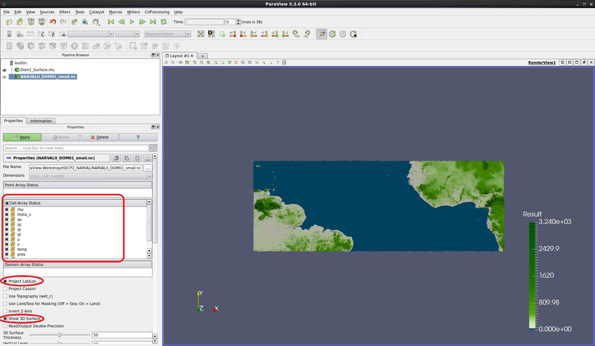
Figure 2: Prior to applying the data,check all cells,Project Lat/LonandShow 3D Surface

This may take a few seconds, as indicated by the blue progress bar below the viewer window. A gray rectangle has appeared (see Fig. 3).

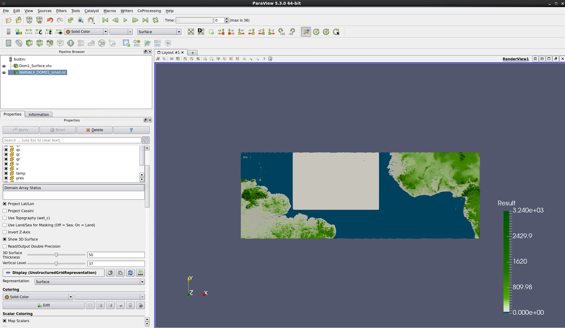
Figure 3: Data as 3D surface applied

With the left mouse button pressed, tilt the data visualization to a view from below (see Fig. 4).

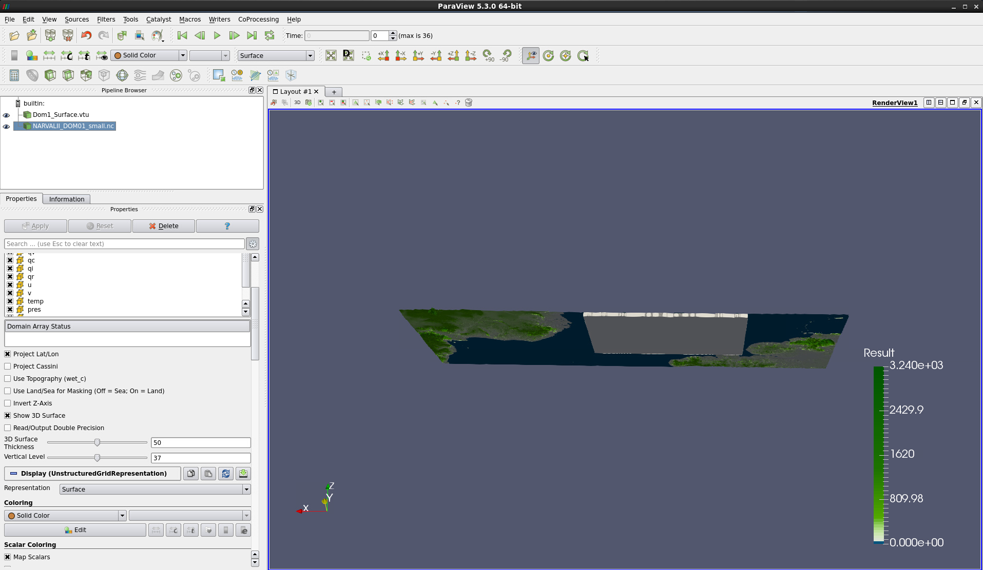
Figure 4: Data as 3D surface seen from below

Now the 3D surface structure of the data becomes obvious. Next, we would like to increase the vertical scale of the data and display the entire 3D volume on top of the map background.

3. In the Properties of the NARVALII_DOM01_small.nc data module:

• Increase 3D Surface Thickness to 500

• Click Apply

See Fig. 5 for details and the result.

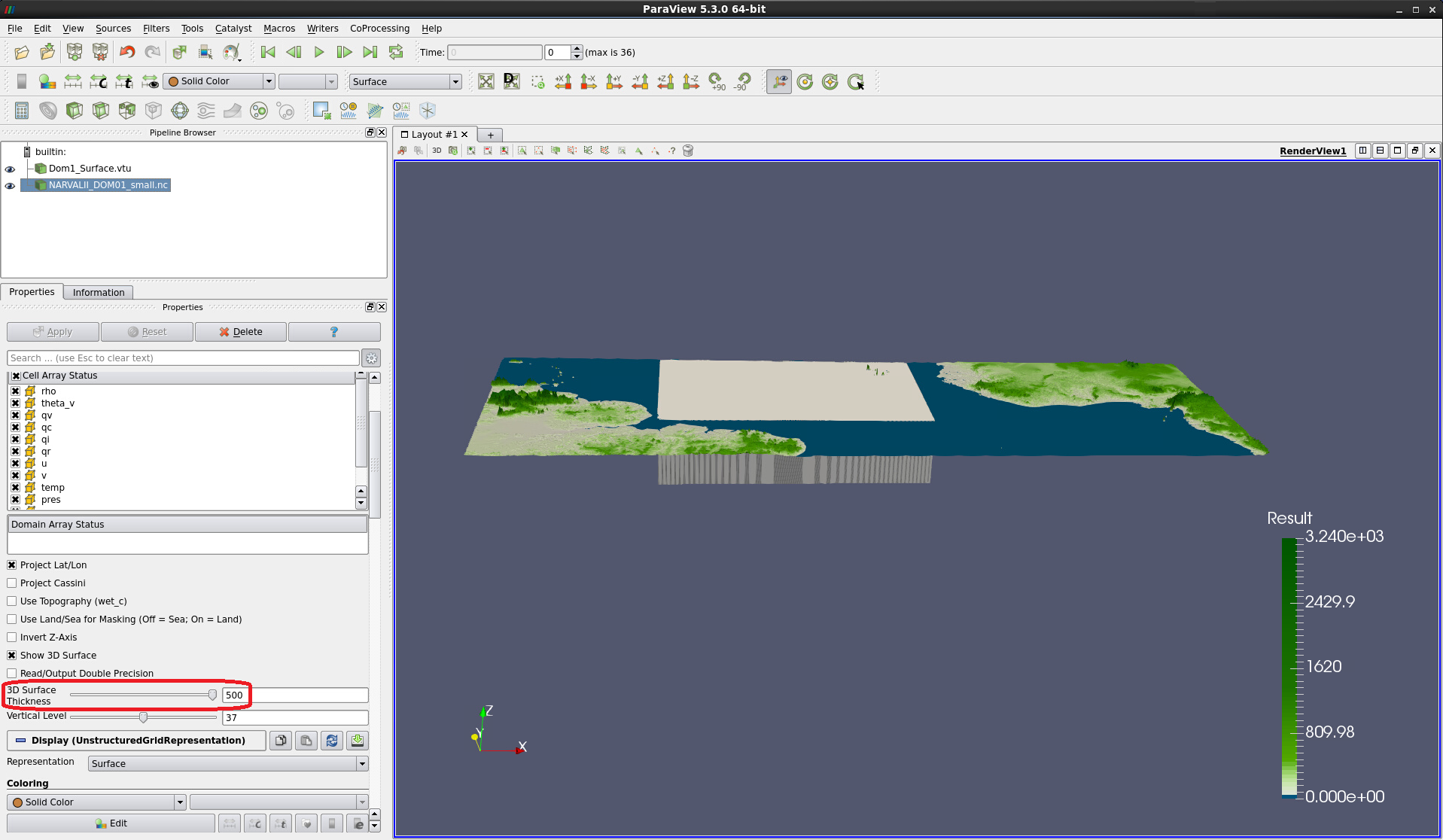
Figure 5: 3D Surface Thickness increased to a value of 500

4. In the Properties of Dom1_Surface.vtu:

• Scroll down to the Transforming section

• Enter -8 into the rightmost box behind Translation

This yields the result shown in Fig. 6.

Figure 6: Background Dom1_Surface.vtu shifted vertically by -8

When looking at the Information tab of the data moduleNARVALII_DOM01_small.nc as shown in Fig. 7, we receive plenty of information on the grid, bounds, time steps, variables and data ranges.

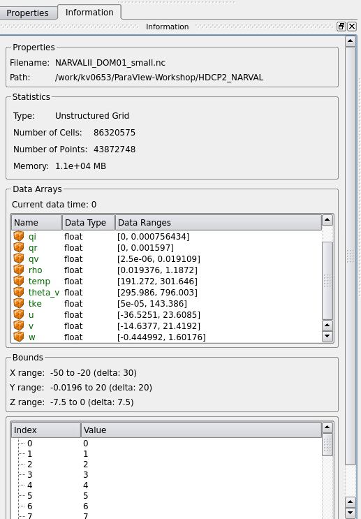
Figure 7: Information on NARVALII_DOM01_small.nc

The cuboid symbol in the list of variables indicates that all variables are cell variables. Wind velocities u, v and w are stored in different variables. Our next step will be to compute the wind vector velocity field. Its magnitude or components can then be used for colorizing the data and for seeding streamlines.

5. Add a Calculator filter:

• With NARVALII_DOM01_small.nc selected, click on the Calculator symbol in the toolbar.

• Change Attribute Mode to Cell data

• Set a Result Array Name, e.g. wind or velocity. In this example we’ll be using wind.

• Enter the formula u*iHat+v*jHat+w*kHat into the input field, combining the separate velocities with their unit vectors.

• Click Apply

6. In the toolbar, click on the little arrow next to Solid Color to see all variables available for coloring the 3D surface. Select the newly created wind.

7. Switch off the colormap legend for the background by selecting Dom1_Surface.vtu and clicking on the leftmost item Toggle Color Legend Visibility. Note that Magnitude is the default representation for wind. However, the X, Y or Z component are available as well for coloring. – See Fig. 8.

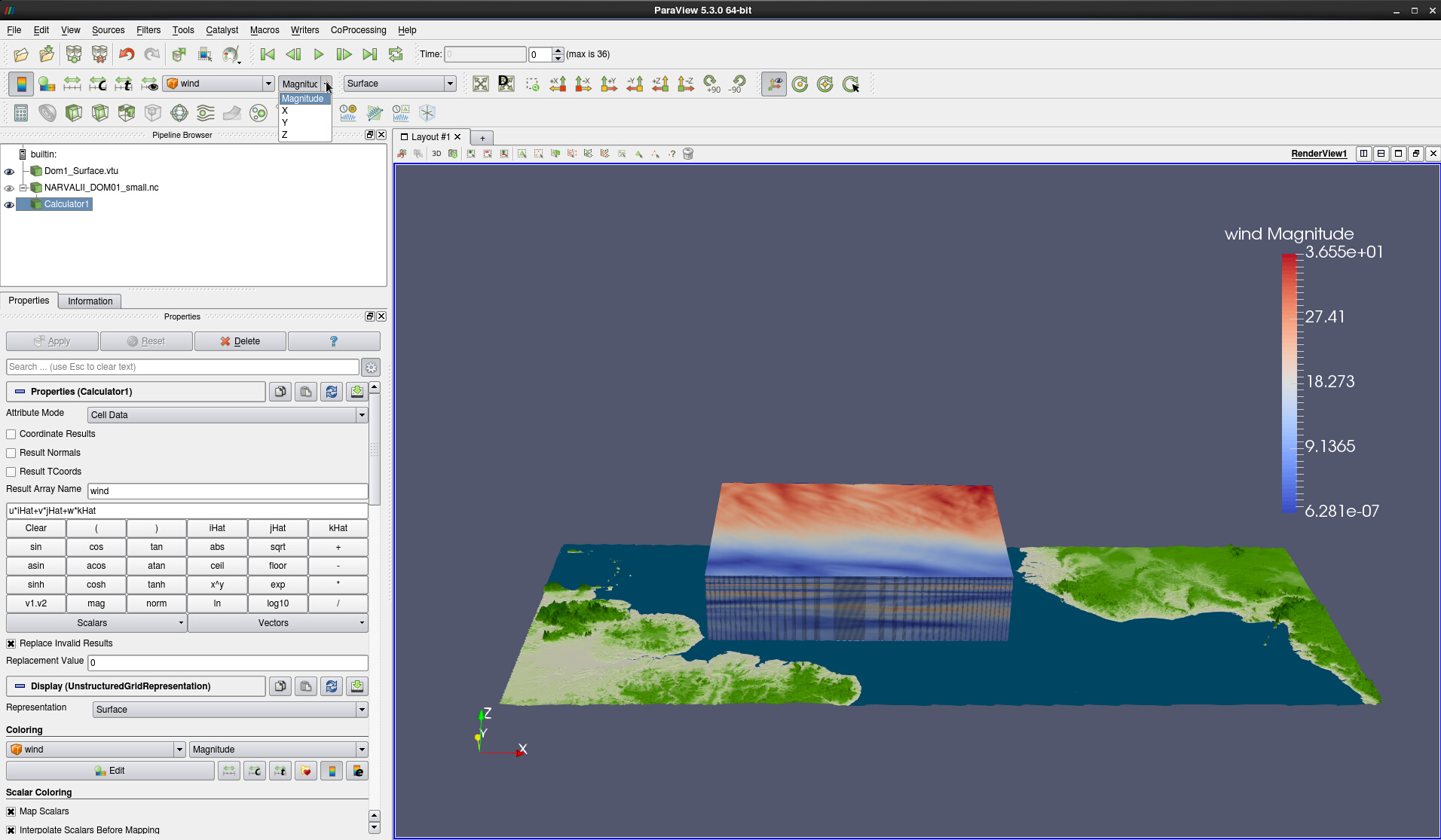
Figure 8: 3D Surface colored by wind magnitude

For the streamline seeding and colorization we need to compute the wind magnitude explicitly: 8. Add a second Calculator filter:

• With Calculator1 selected, add another Calculator filter

• Select Attribute Mode Cell Data

• Call the resulting array e.g. windmag

• Enter mag(wind) in the calculator input field

• Click Apply

Note that the coloring variable in Calculator2 has automatically changed to windmag (see Fig. 9). Our next goal is to identify a hurricane at time step 35 by moving a horizontal slice vertically through the data volume. The area around this hurricane shall then be used as the source area for streamline seeding.

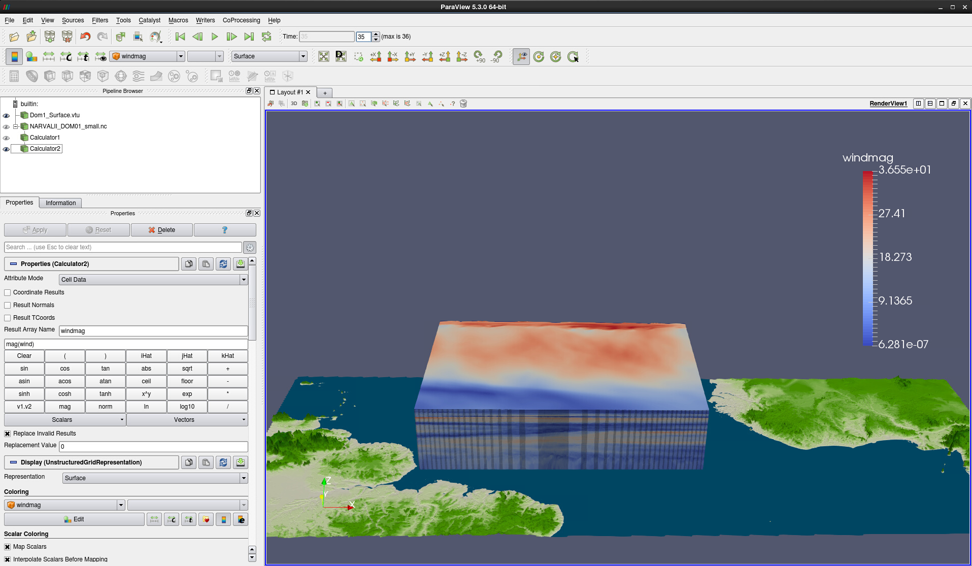
Figure 9: 3D Surface colored by wind magnitude at time step 35

9. In the topmost toolbar, change the Time value to 35.

10. Add a Slice filter to the Calculator2 output

• With Calculator2 selected click on the Slice filter in the toolbar (4th symbol from the left).

• Keep Slice type Plane

• Click on Z Normal

• Drag the slice to a vertical position of your choice

• Click Apply

To identify the hurricane we suggest that you try values between -7 and -6 for the rightmost Origin field in the Plane Parameters (see Fig. 10).

11. With Calculator2 selected, click on the Stream Tracer symbol (highlighted in Fig. 10) in the toolbar.

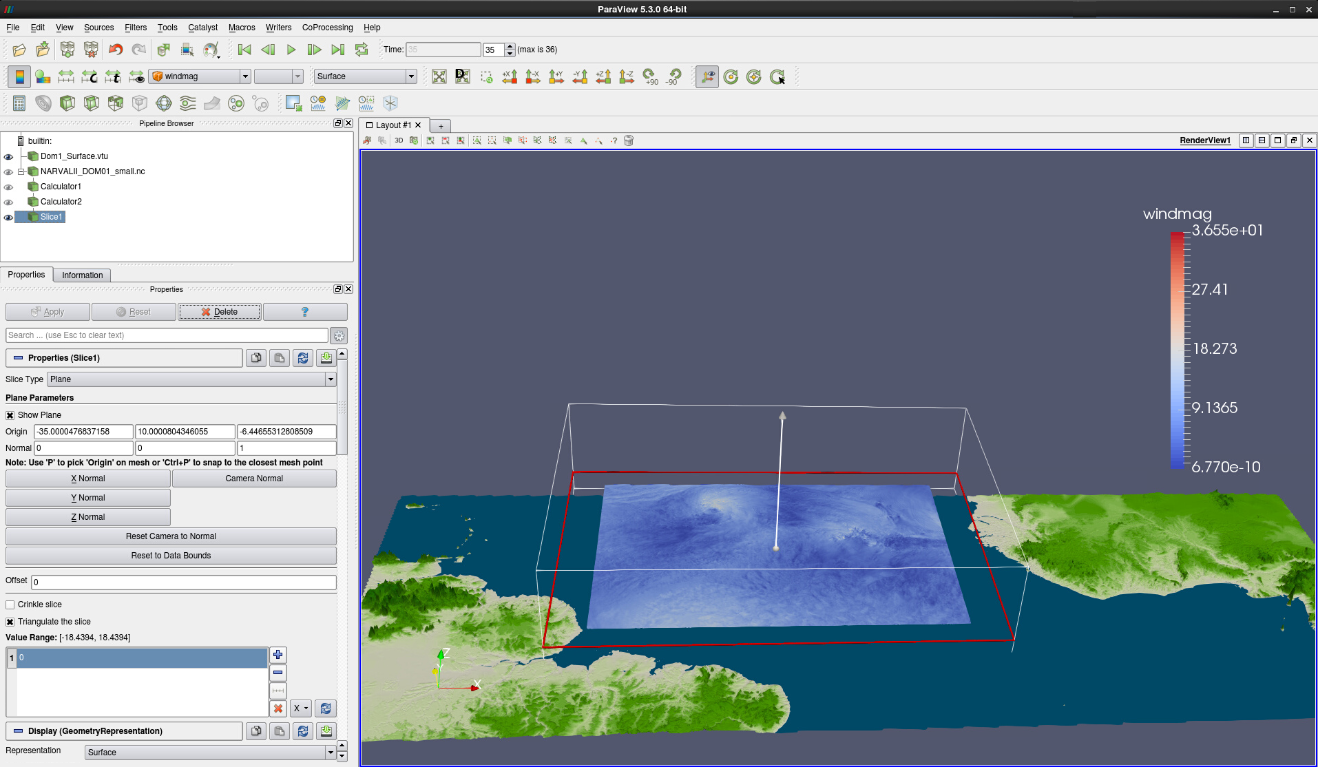
Figure 10: Slice and slicing plane outlining the hurricane by elevated wind magnitude values

Note that two unobtrusive white handles have appeared at two diagonally opposite corners of the data volume. These belong to the default Seed Type High Resolution Line Source, which we will change in a second. 12. In the Stream Tracer Properties, change the Seed Type to Point Source 13. With the left mouse button pressed down, move the Point Source to the hurricane location 14. Keep the other default settings for now and click on Apply ** 15. **Switch off the visibility of Slice1 and select a view from the side. Compare with Fig. 11.

Figure 11: Streamlines seeded by point source above hurricane

16. Instead of Solid Color, select wind (point variable) for coloring.

Looking at Fig. 11 we notice that the Point source is either a bit too small or needs to be positioned lower to better catch the hurricane.

17. In the Sphere Parameters, change the rightmost value of Center to -6

18. Change the colormap as you did for the land background:

• In The Coloring section, click on Edit Color Map

• In the Color Map Editor, click on Choose Preset

• Select, e.g., colormap Black, Orange and White

• Click Apply

• Click Close

• In the Color Map Editor, click on Rescale to Custom Range

• Enter a minimum value of 0 and a maximum value of 20

• Click on Rescale

This looks a bit better already. We suggest changing the appearance of the colormap legend min and max values and also the title. 19. Change the color map legend:

• Clicking on Edit color legend properties, the button in the top right corner of the Color Map Editor

• Change the Range Label Format to %2.0f

• In the Title Texts section, you may write Wind with capital W and add the unit [m/s] behind Magnitude in the Component title (see Fig. 12).

• Click Apply

• Click OK

• Close the Color Map Editor

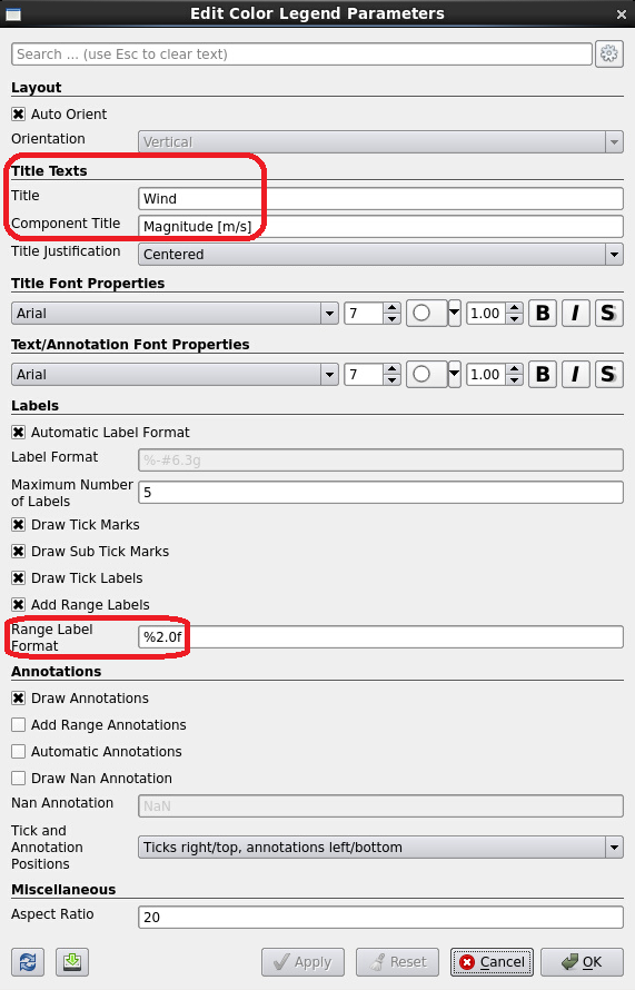
Figure 12: Editing the color legend properties

Last but not least we suggest shortening the streamlines a bit to get a better view of the hurricane structure. 21. In the Stream Tracer1 Properties: - Uncheck Show Sphere – We are fine with the current seed position - Change the Maximum Stream Line Length to 10 (compare Fig. 13) - You may also want to try modifying other settings – such as decreasing the Number of Points to 50 (compare Fig. 14).

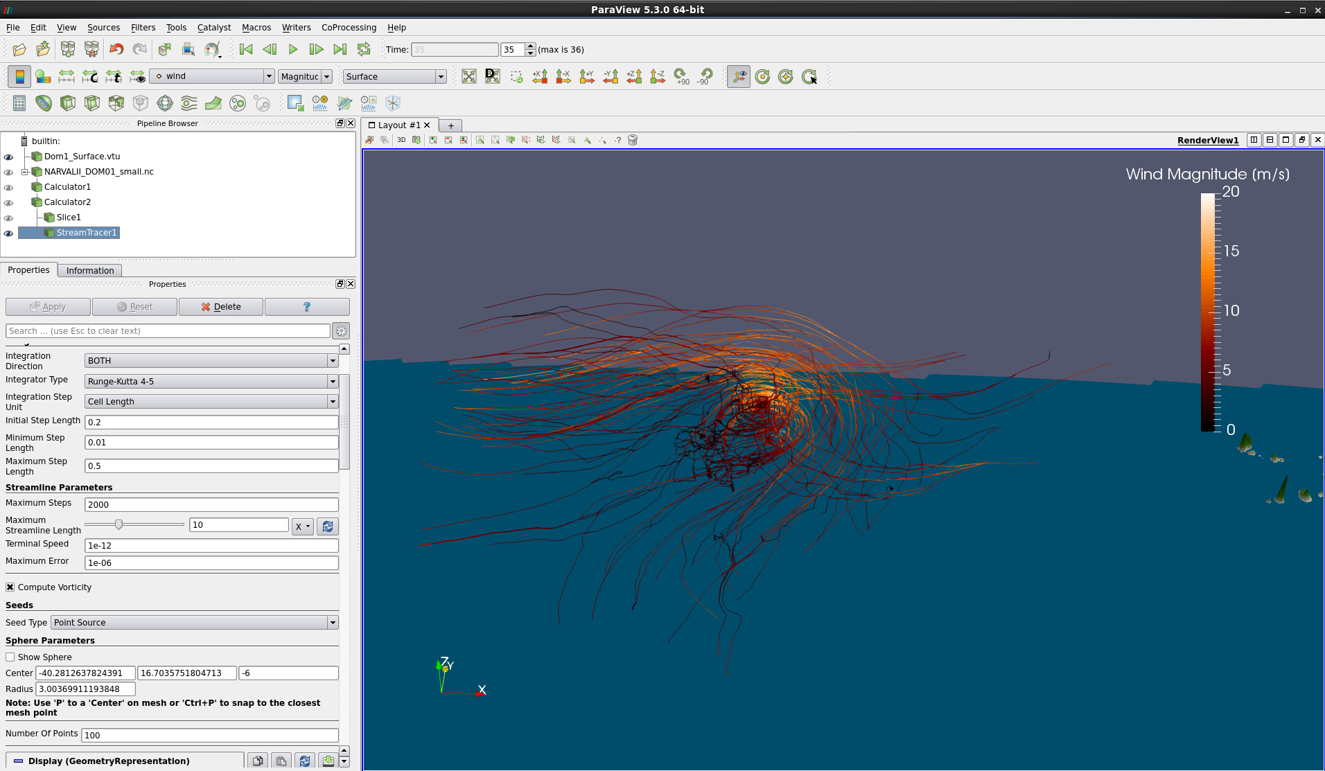
Figure 13: 100 streamlines of length 10 seeded in hurricane region and colored by wind magnitude

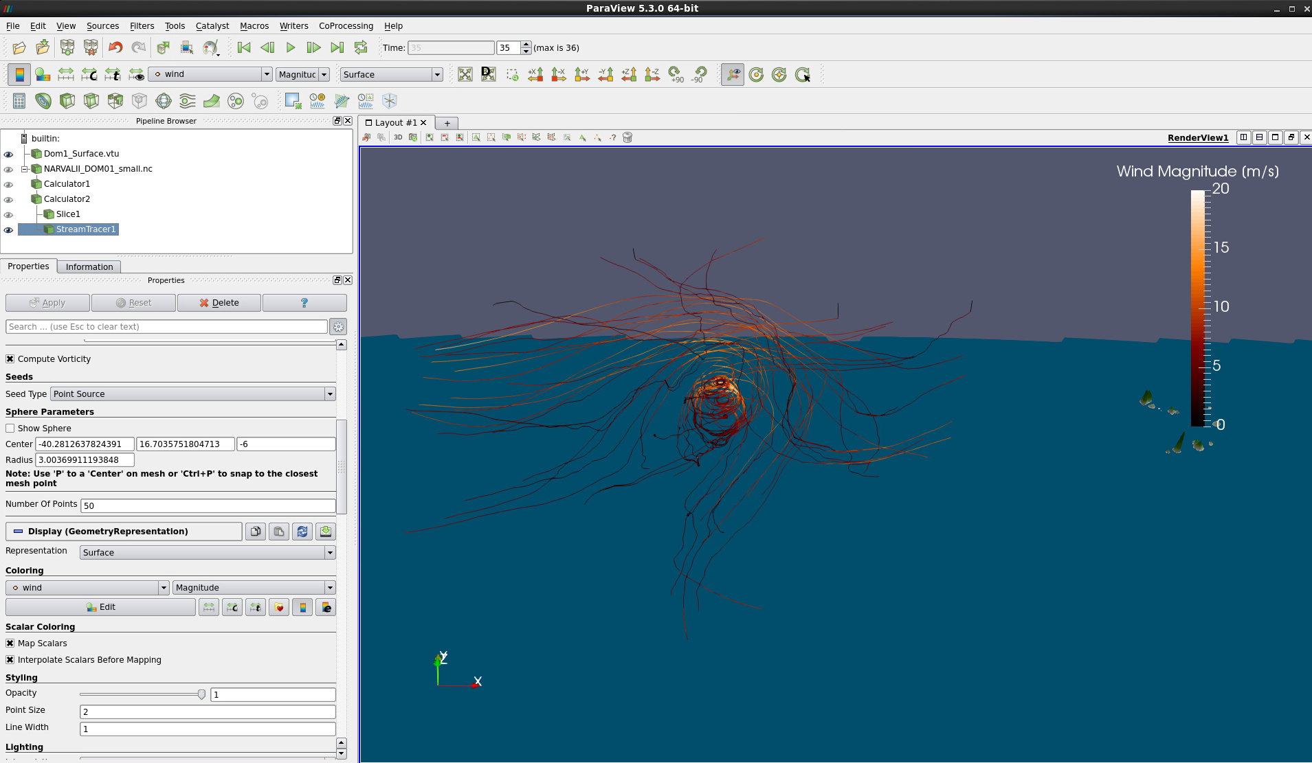
Figure 14: 50 streamlines of length 10 seeded in hurricane region

Please note that it is not possible to increase the streamline diameter. An option is applying an additional Tube or Ribbon filter to the Stream Tracer output. Moreover, a number of secondary variables such as gradients and vorticity can be derived from the input data. However, as these tasks are more complex and require further filter operations, they are not part of this introductory how-to.