NCL examples#
Most of the NCL examples, tipps and tricks have been collected from our NCL user requests. The special examples are developed at DKRZ to support our users and to demonstrate NCL’s capabilities (here NCL version 6.4.0). The used data sets of the example scripts are stored on our supercomputer mistral in the directory /work/kv0653/NCL/data_examples.
Categories#
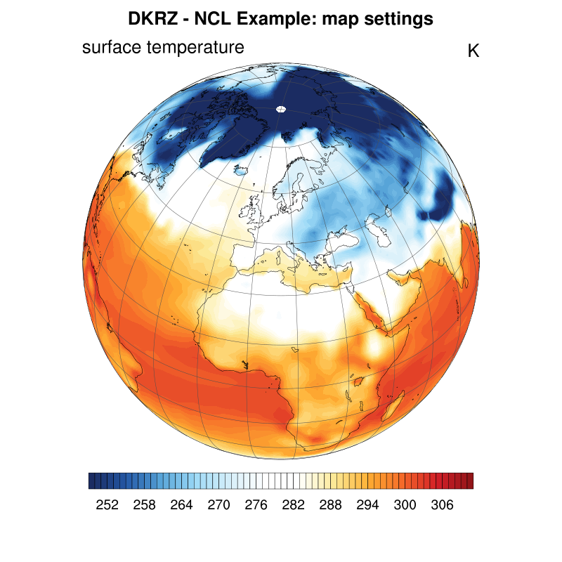
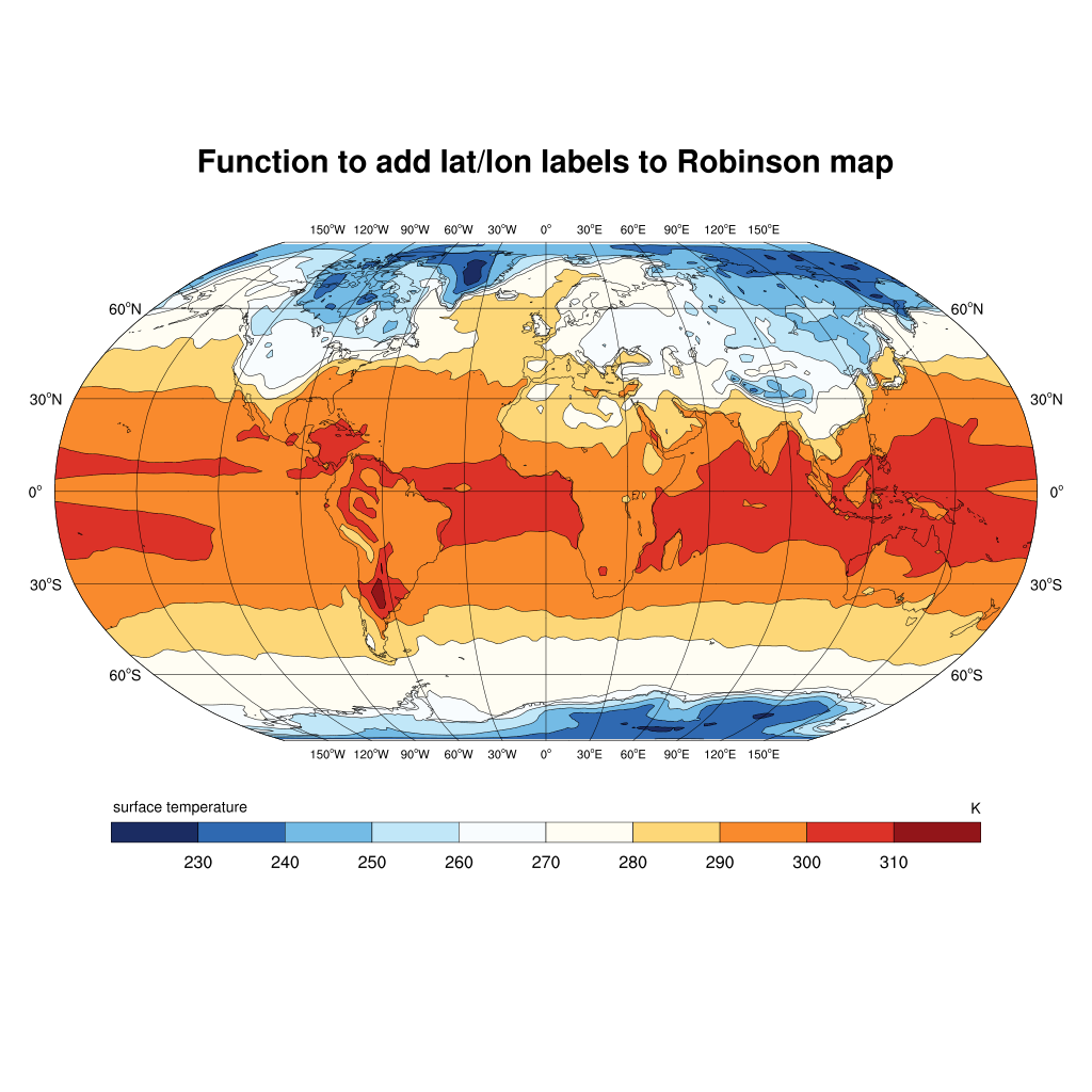
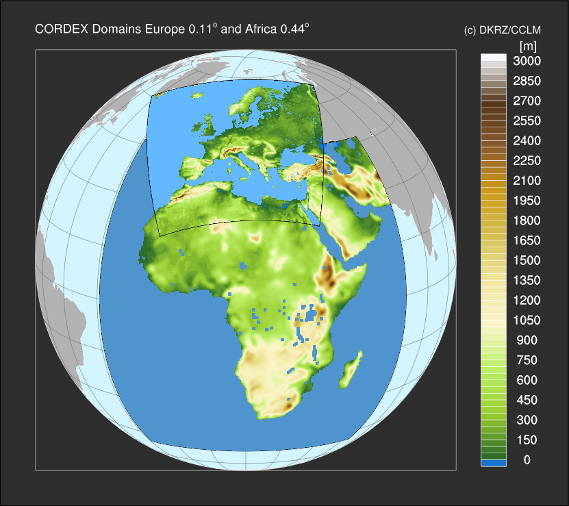
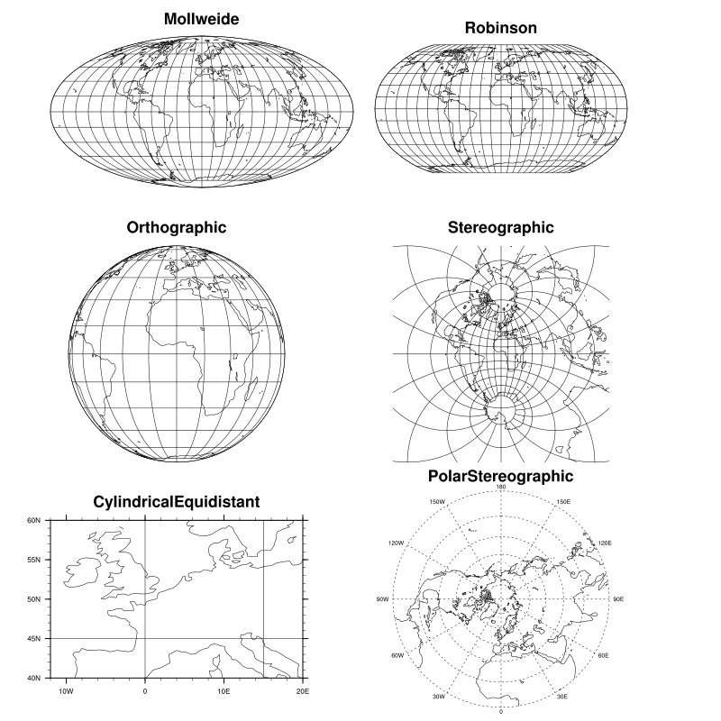
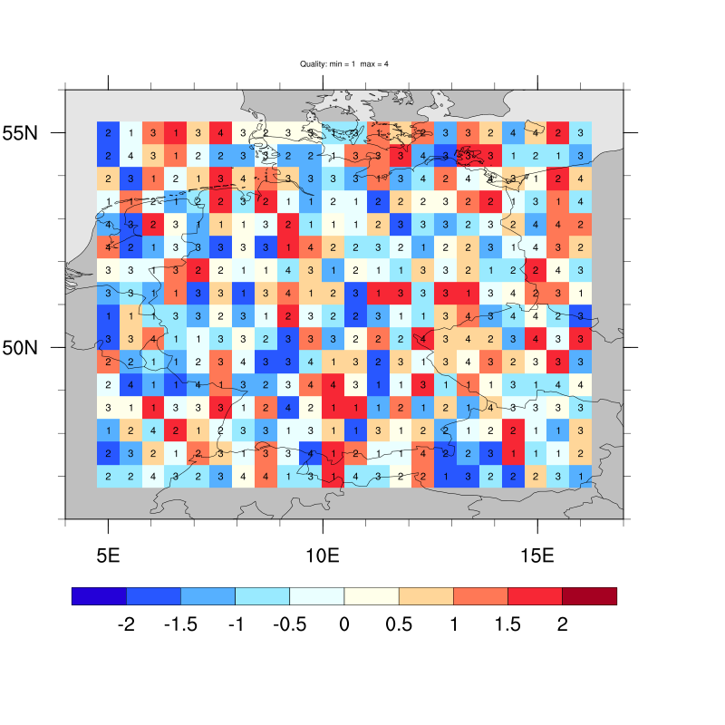
map resources, functions, select sub-region, overlays, coastal outlines, map areas |
|
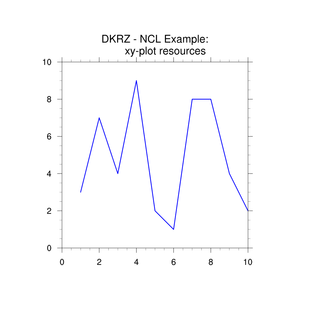
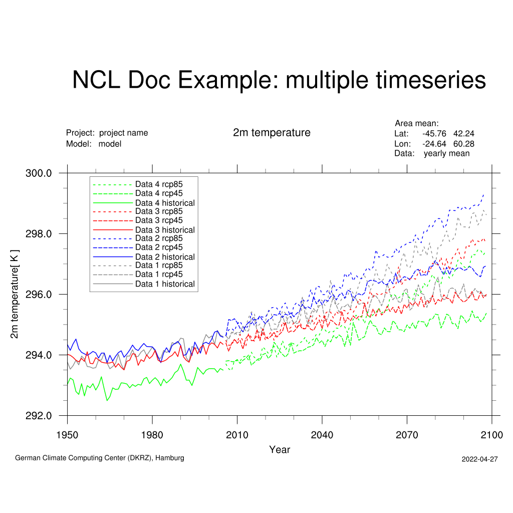
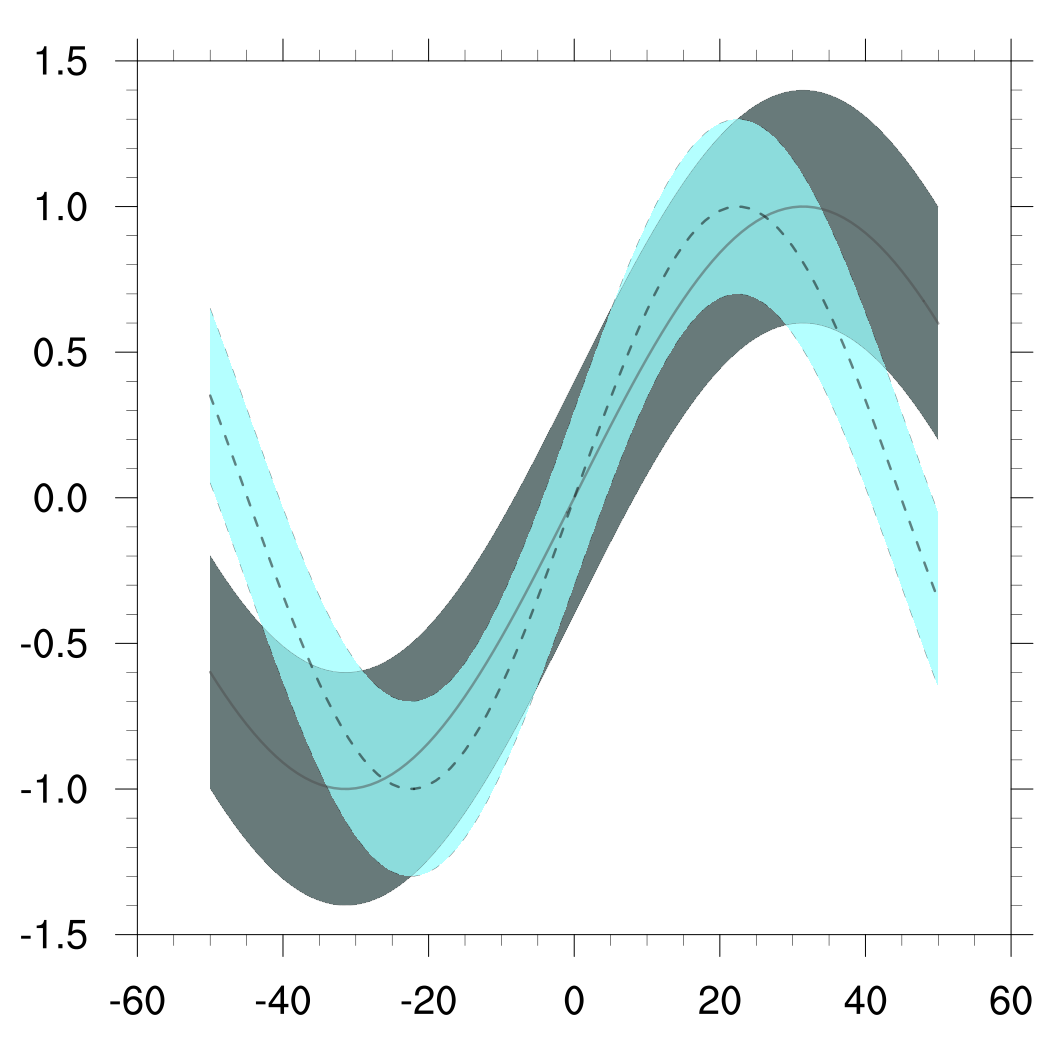
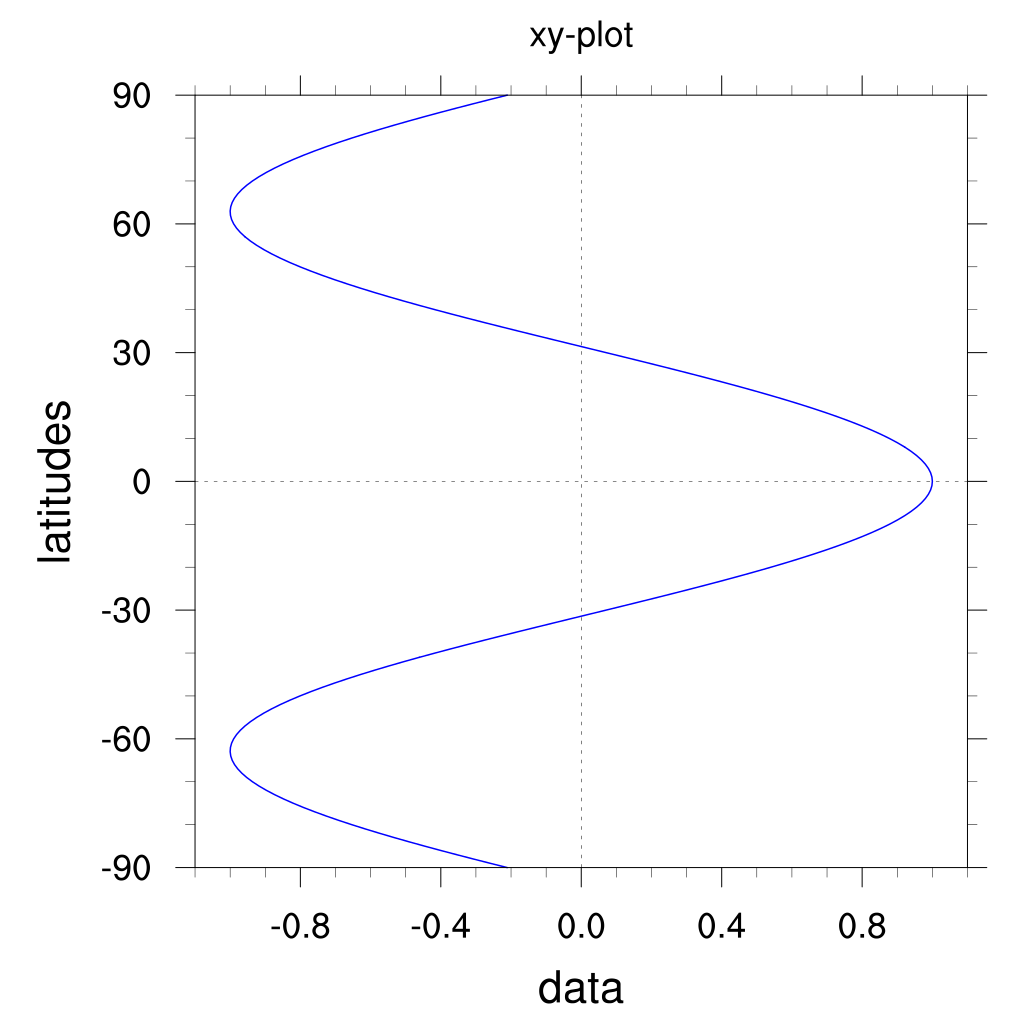
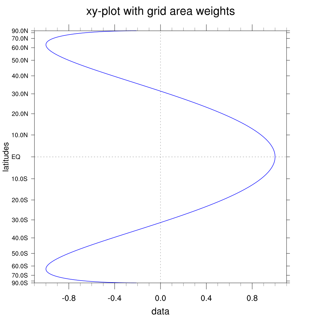
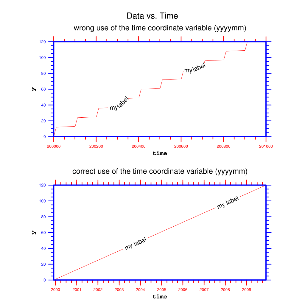
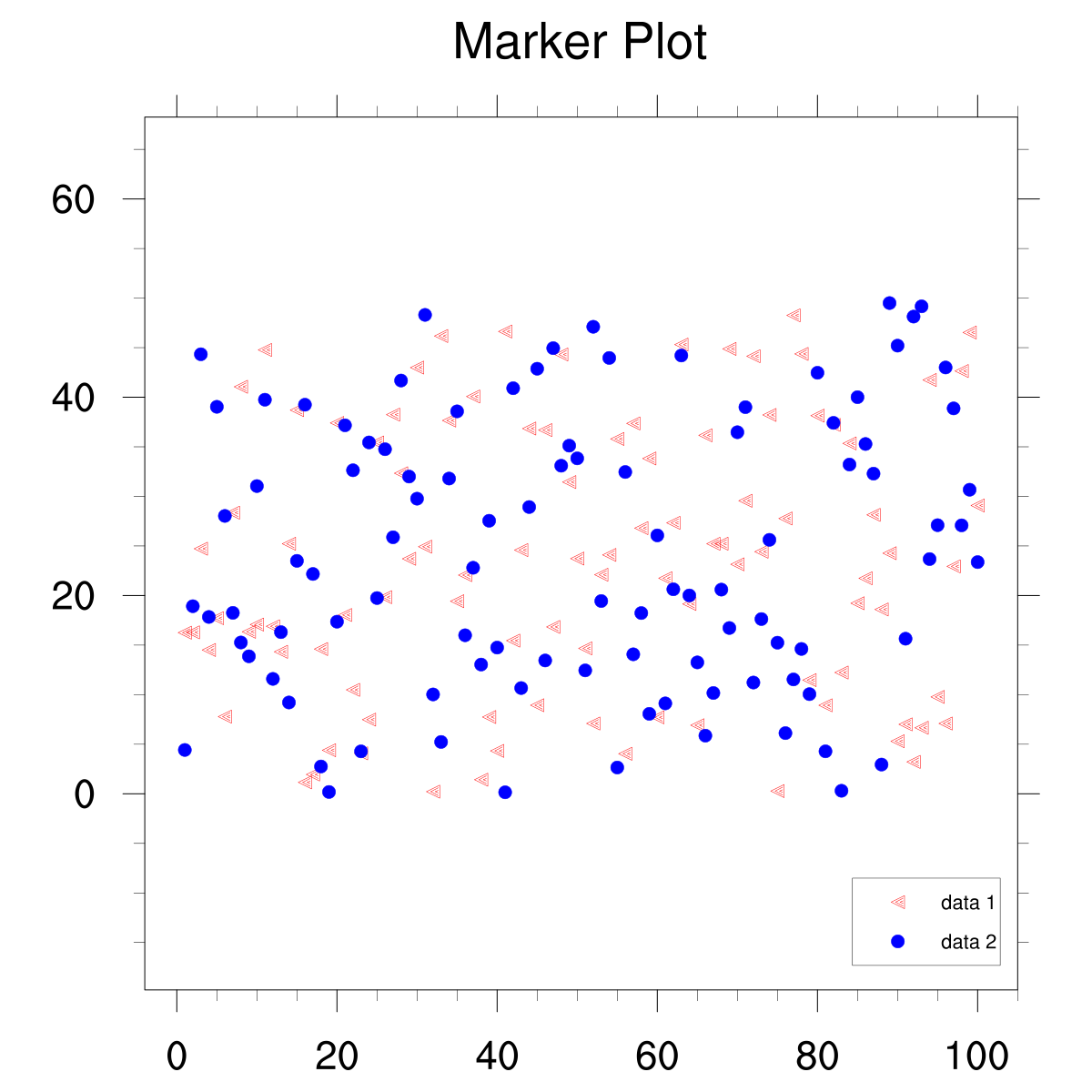
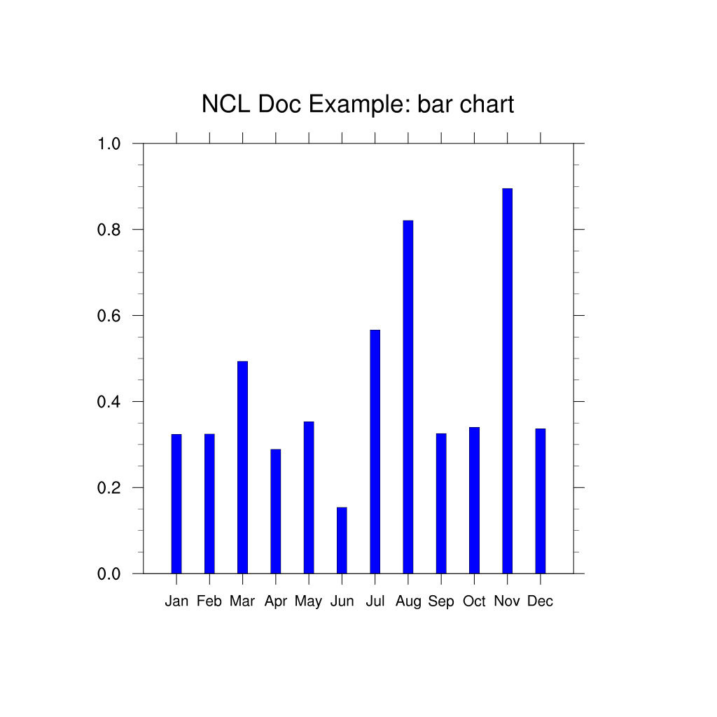
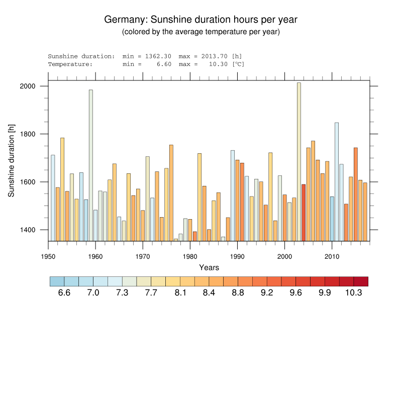
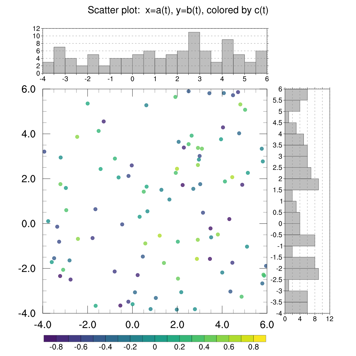
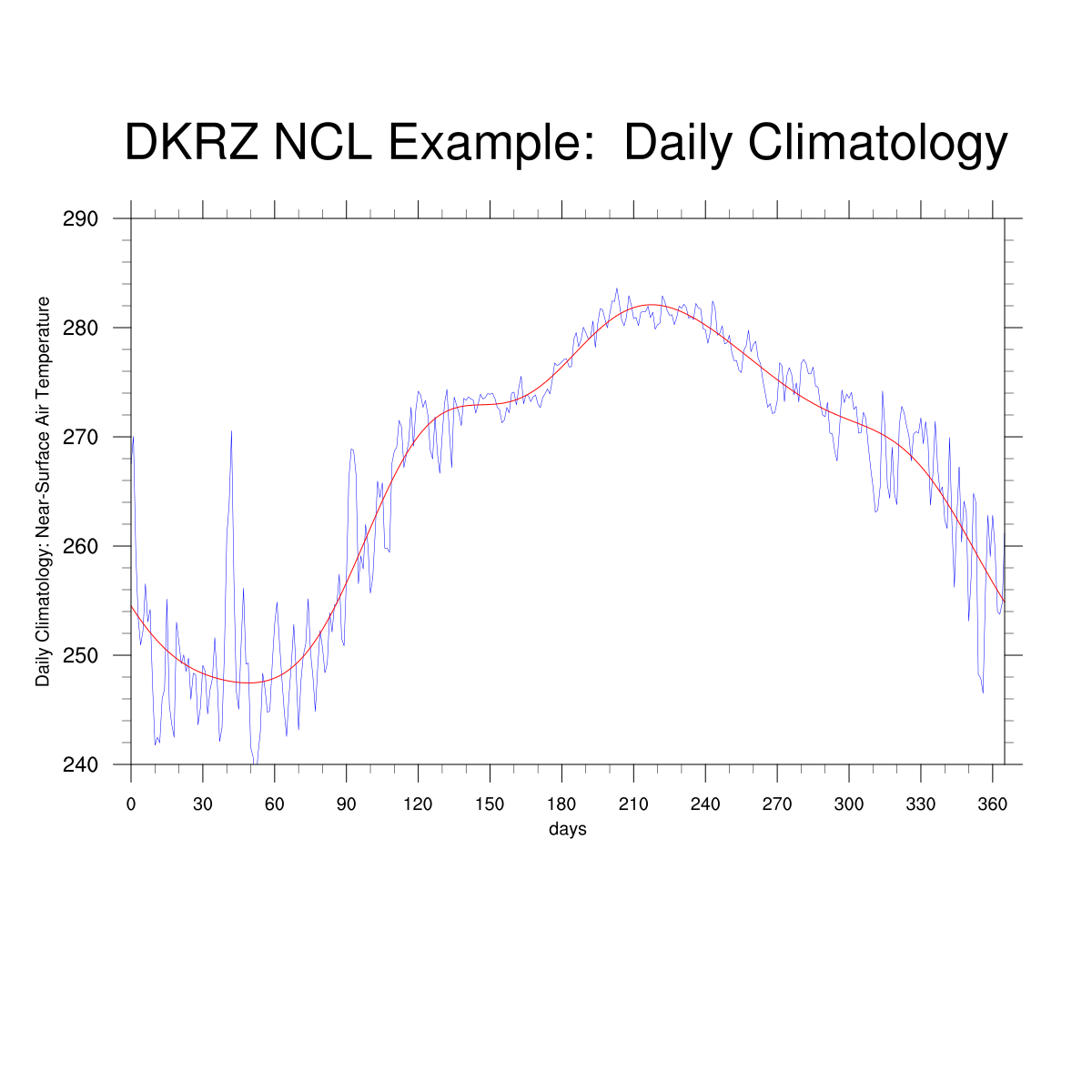
1D data line plot, timeseries, statistics |
|
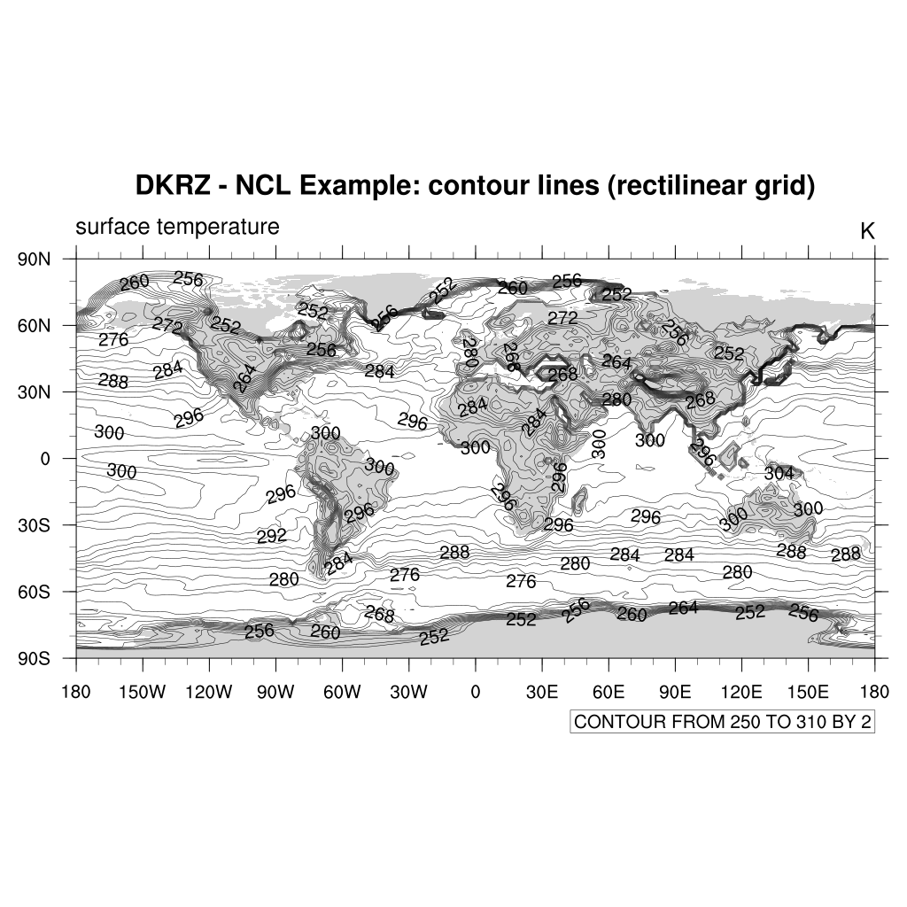
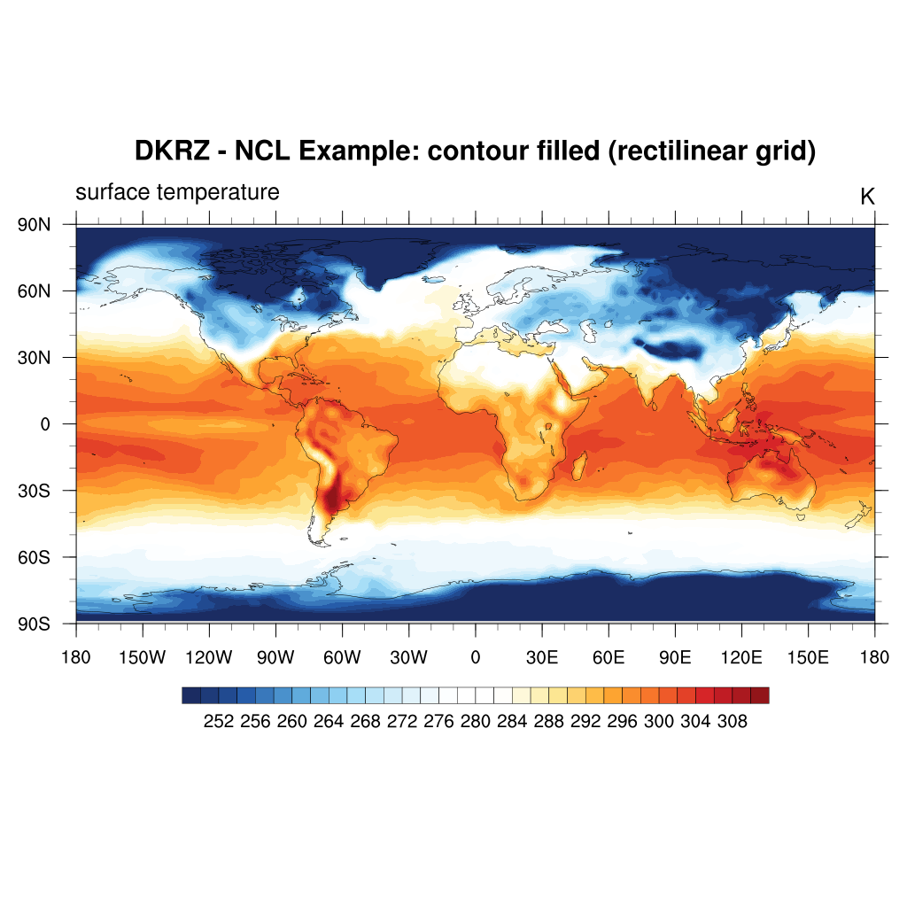
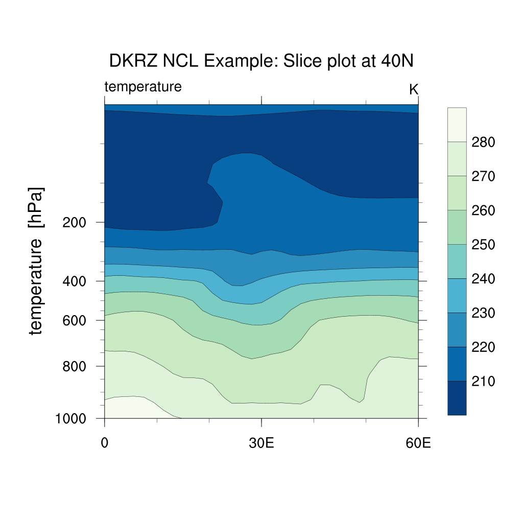
2D data line, color fill (shaded), fill pattern, overlays, slices |
|
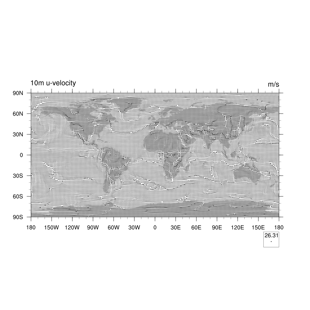
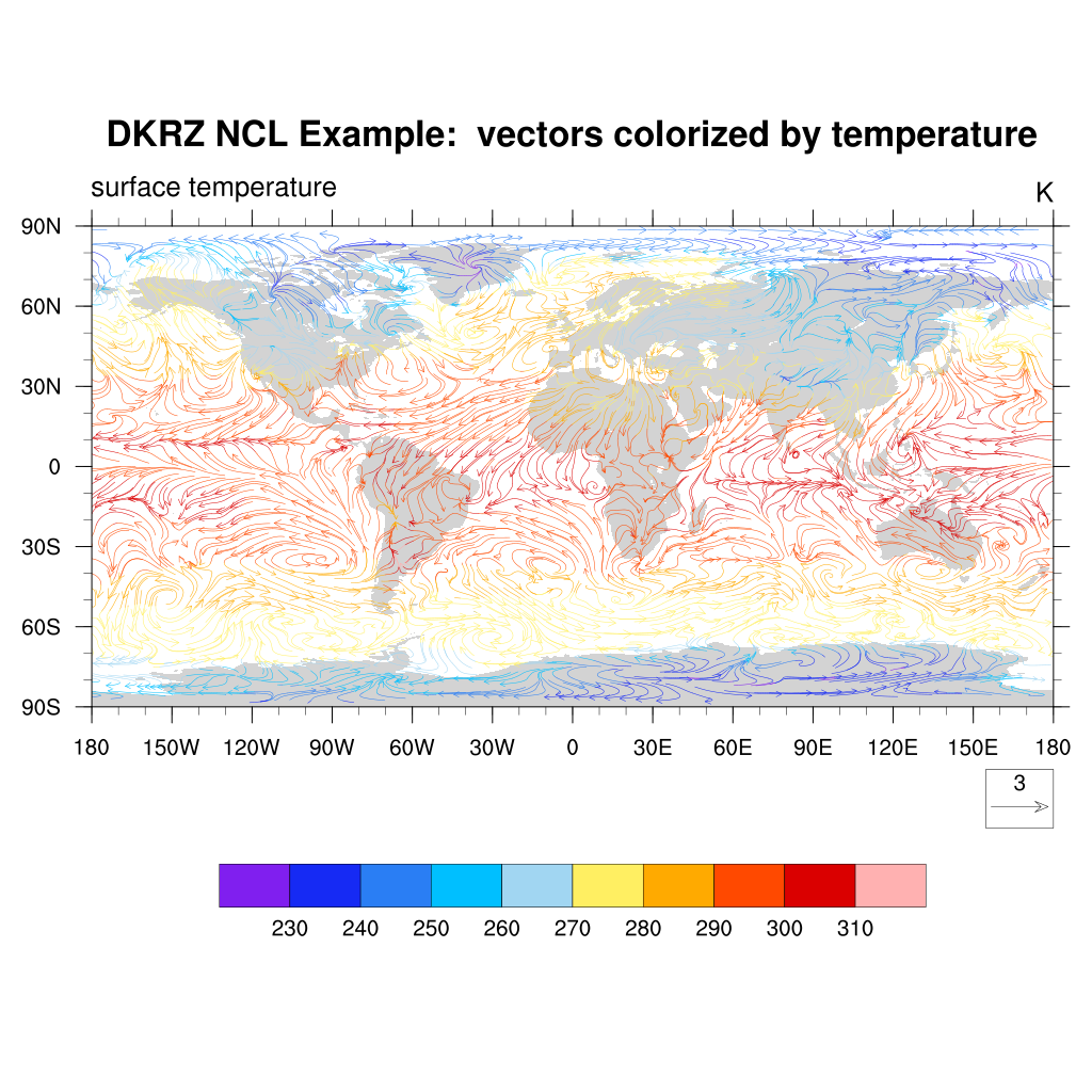
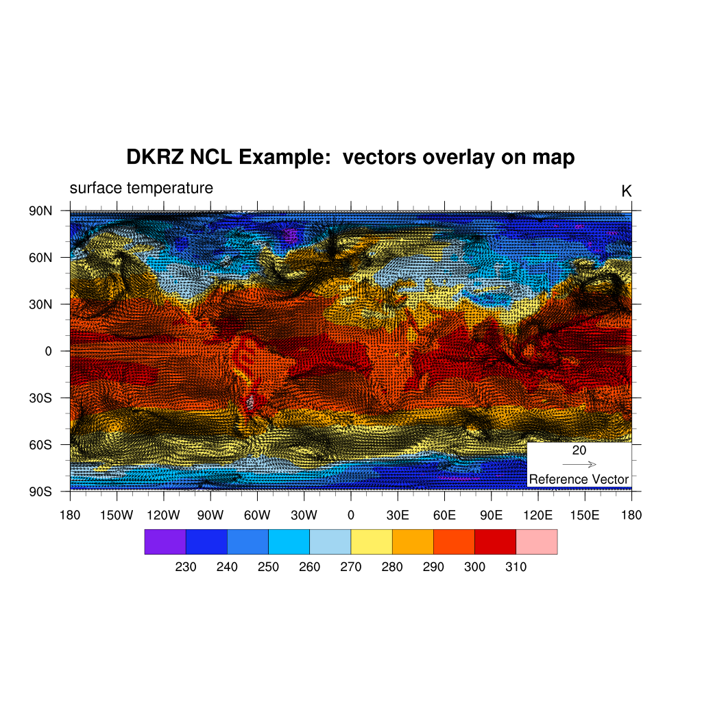
2D vector data, e.g. wind components uv |
|
contour line on filled contour plot, vector on contours, different grid resolutions |
|
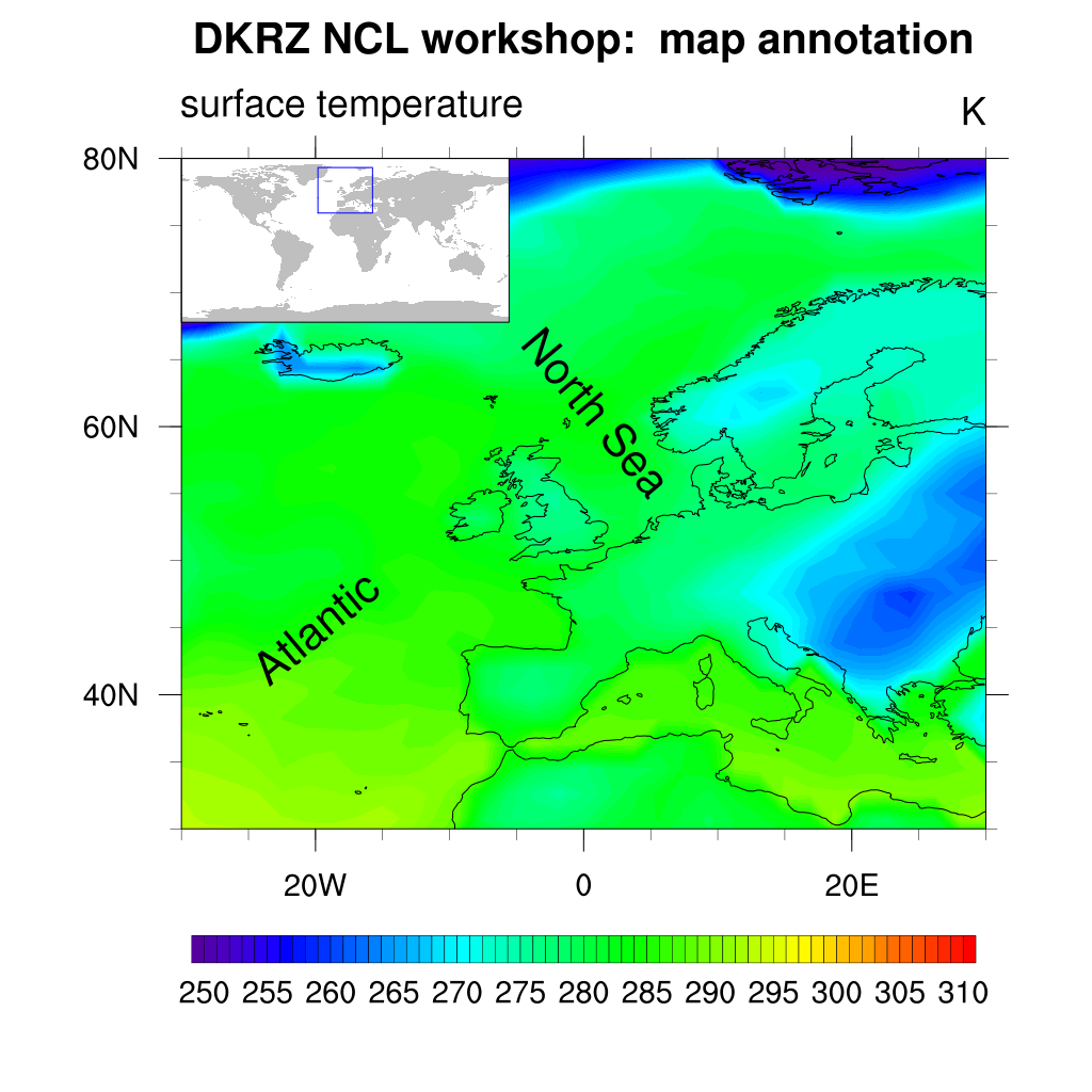
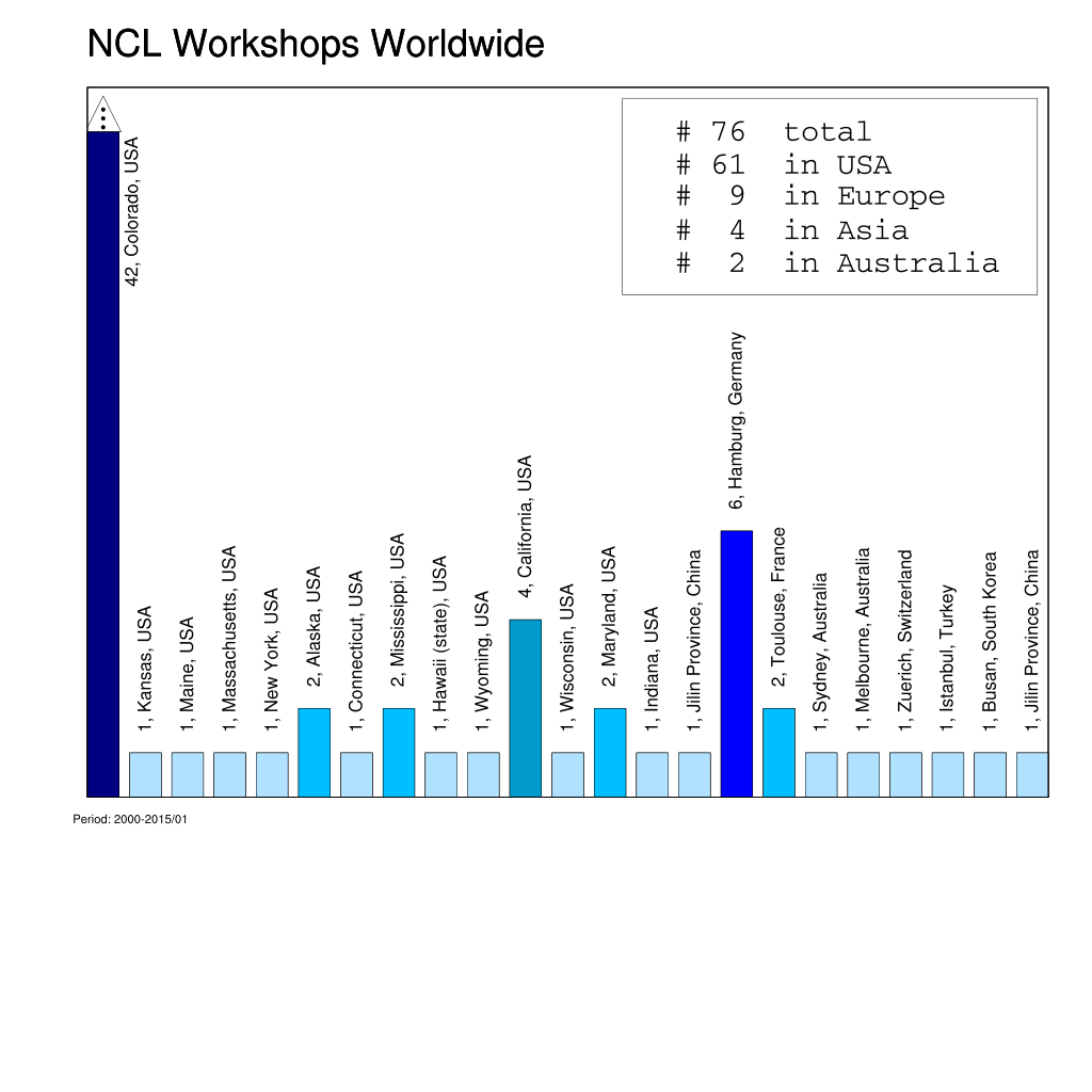
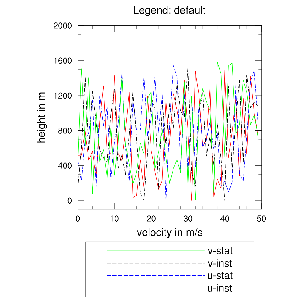
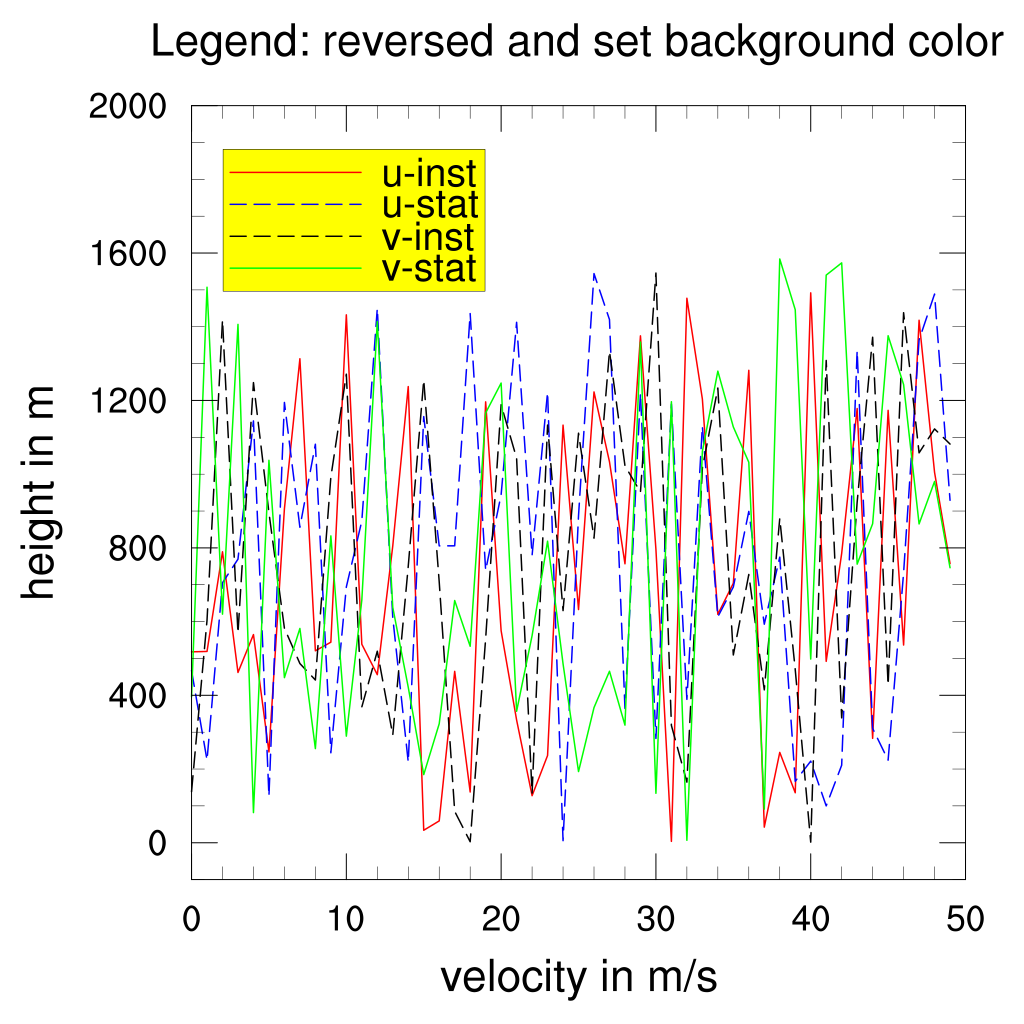
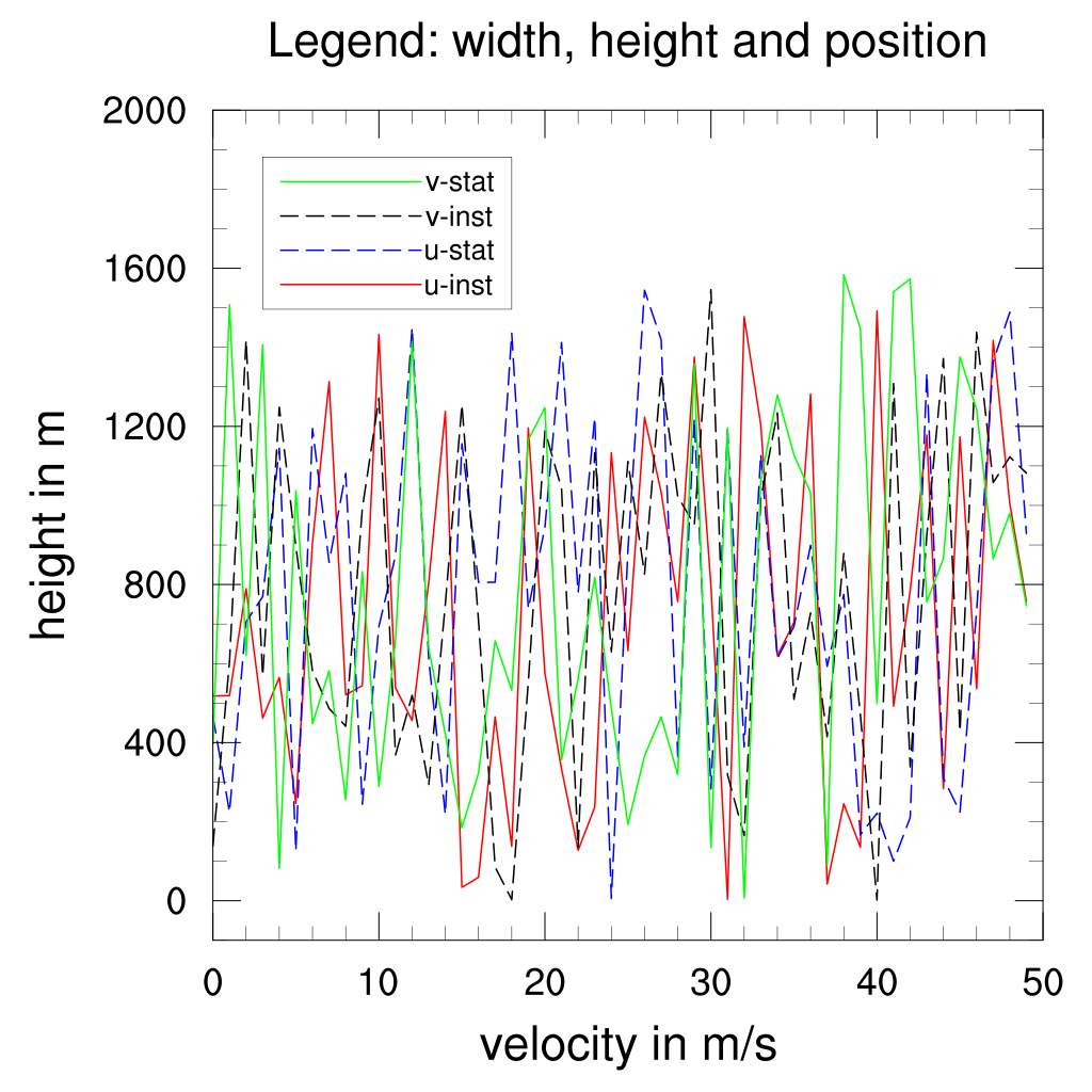
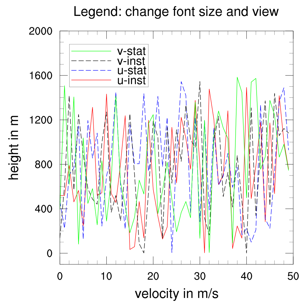
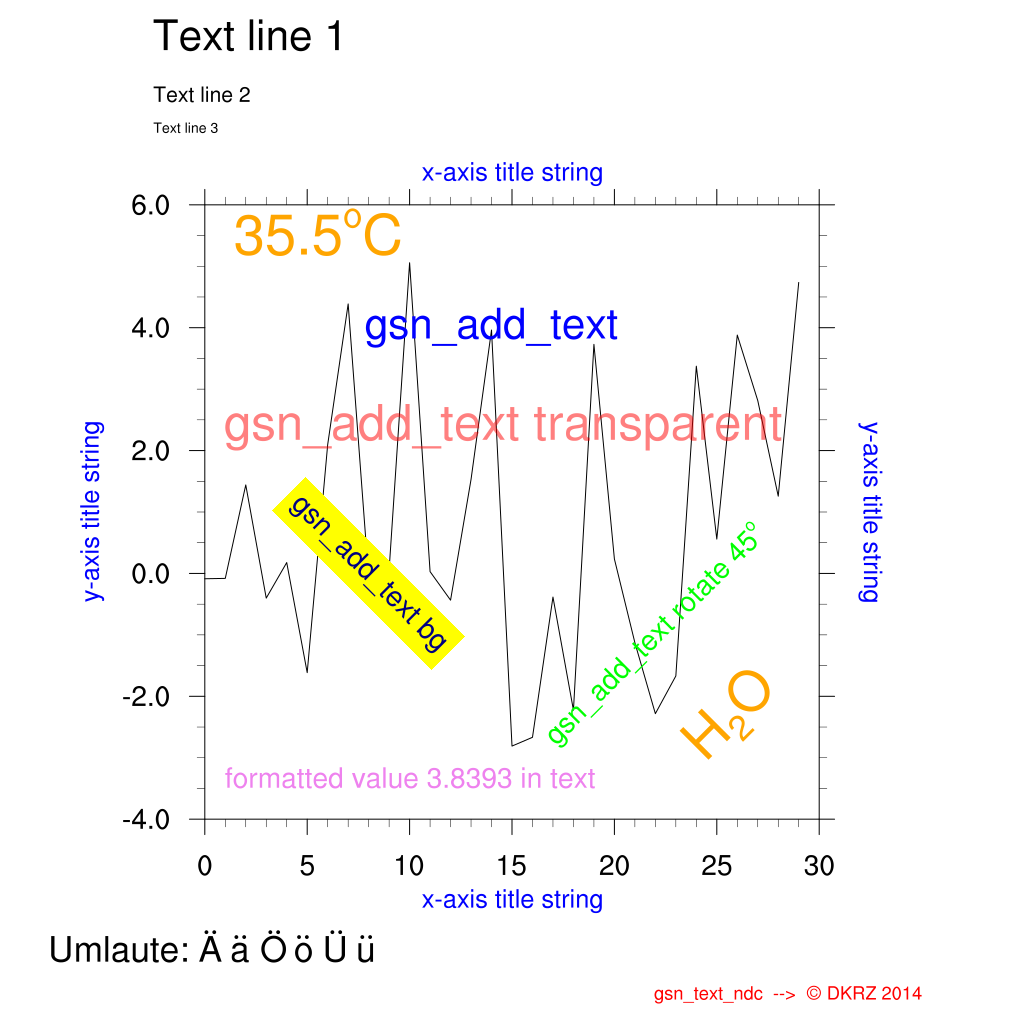
annotations, e.g. text, legends, labelbars, maps, plots |
|
multiple plots in one frame (page) |
|
time depending animations, create single plot for each timestep |
|
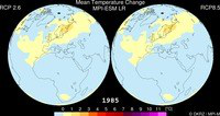
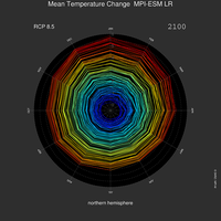
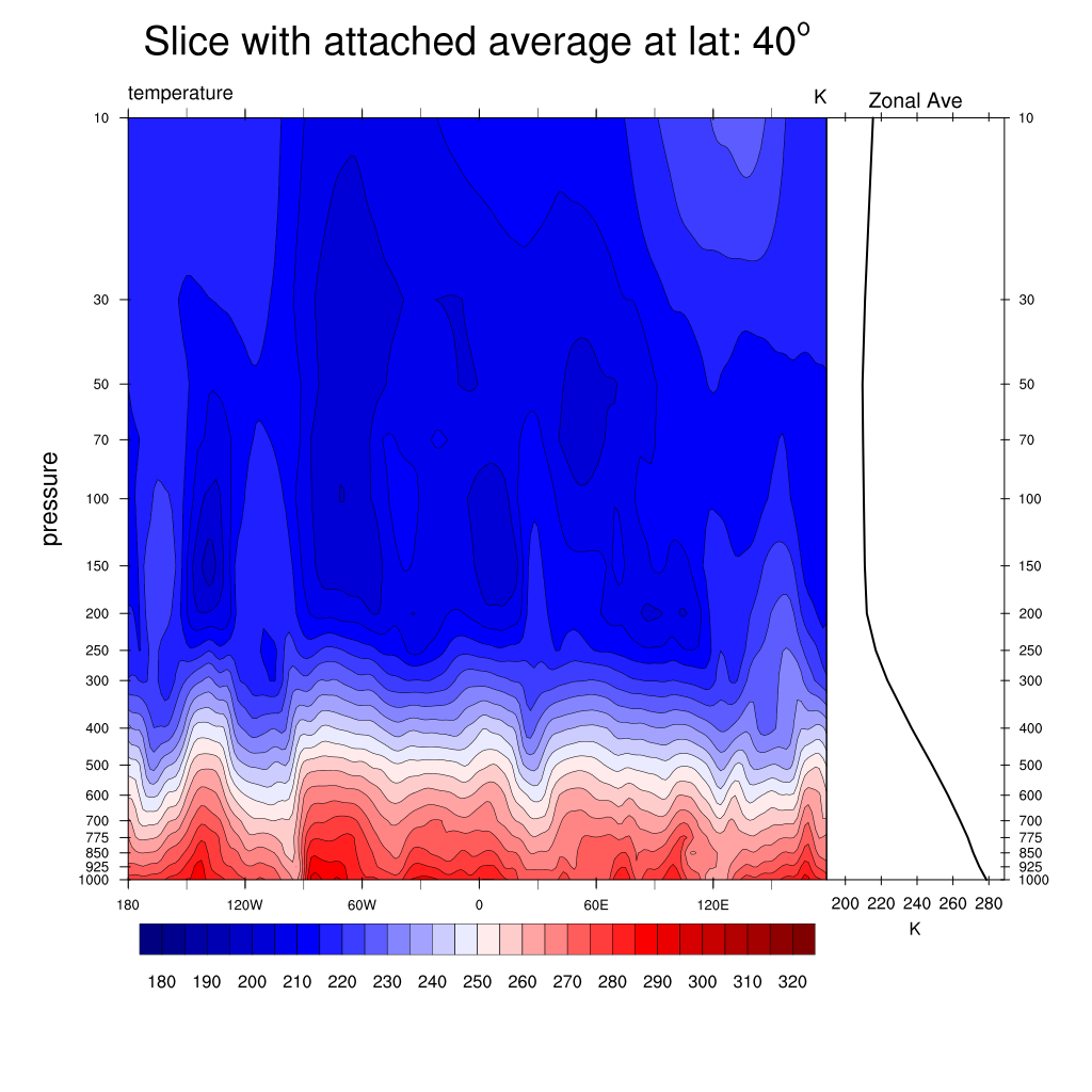
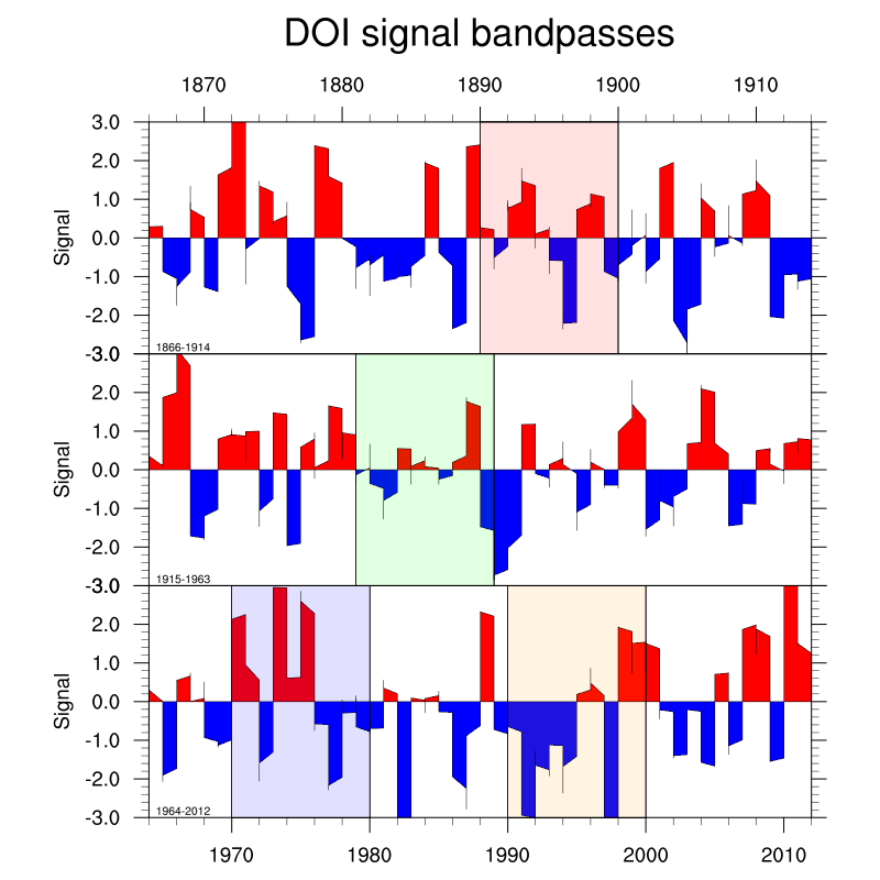
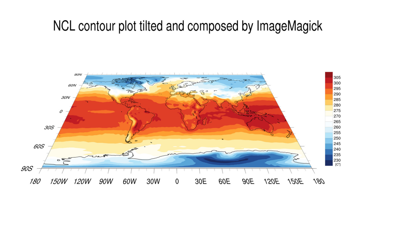
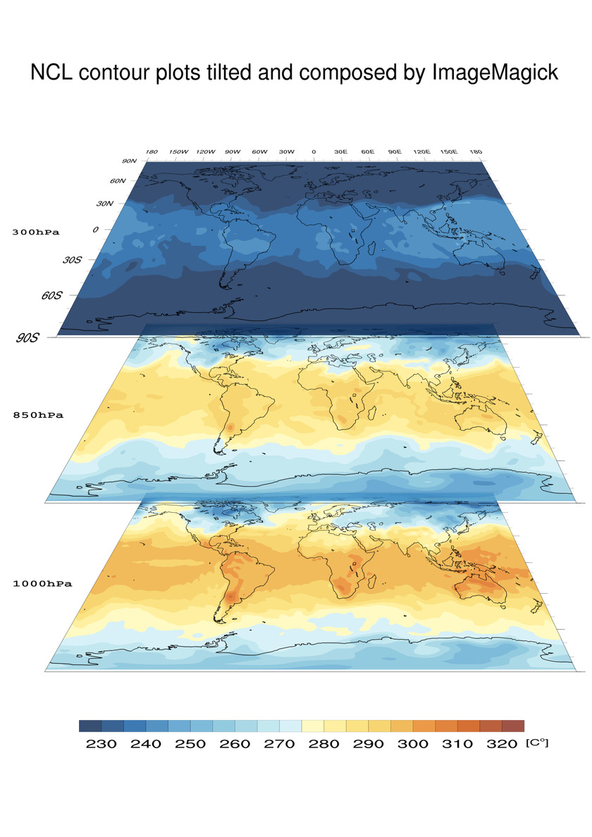
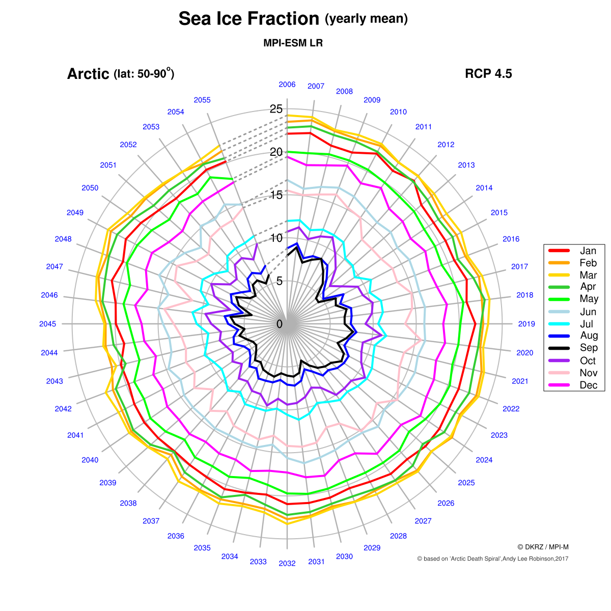
attach plot along y-axis, plot long timeseries, clouds and labelbar with transparency, map areas, spiral plot (Ed Hawkins), simulate 3D view, tilt contour plots using ImageMagick |
|
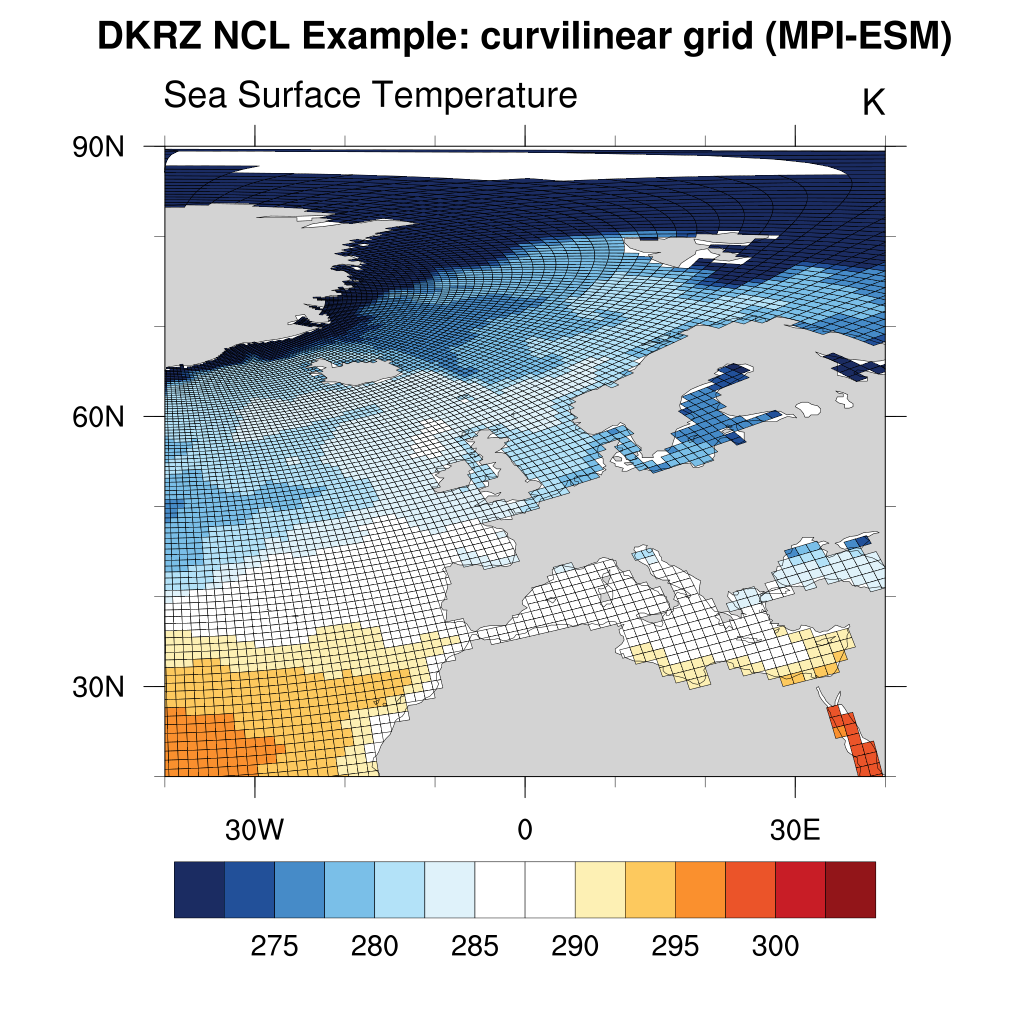
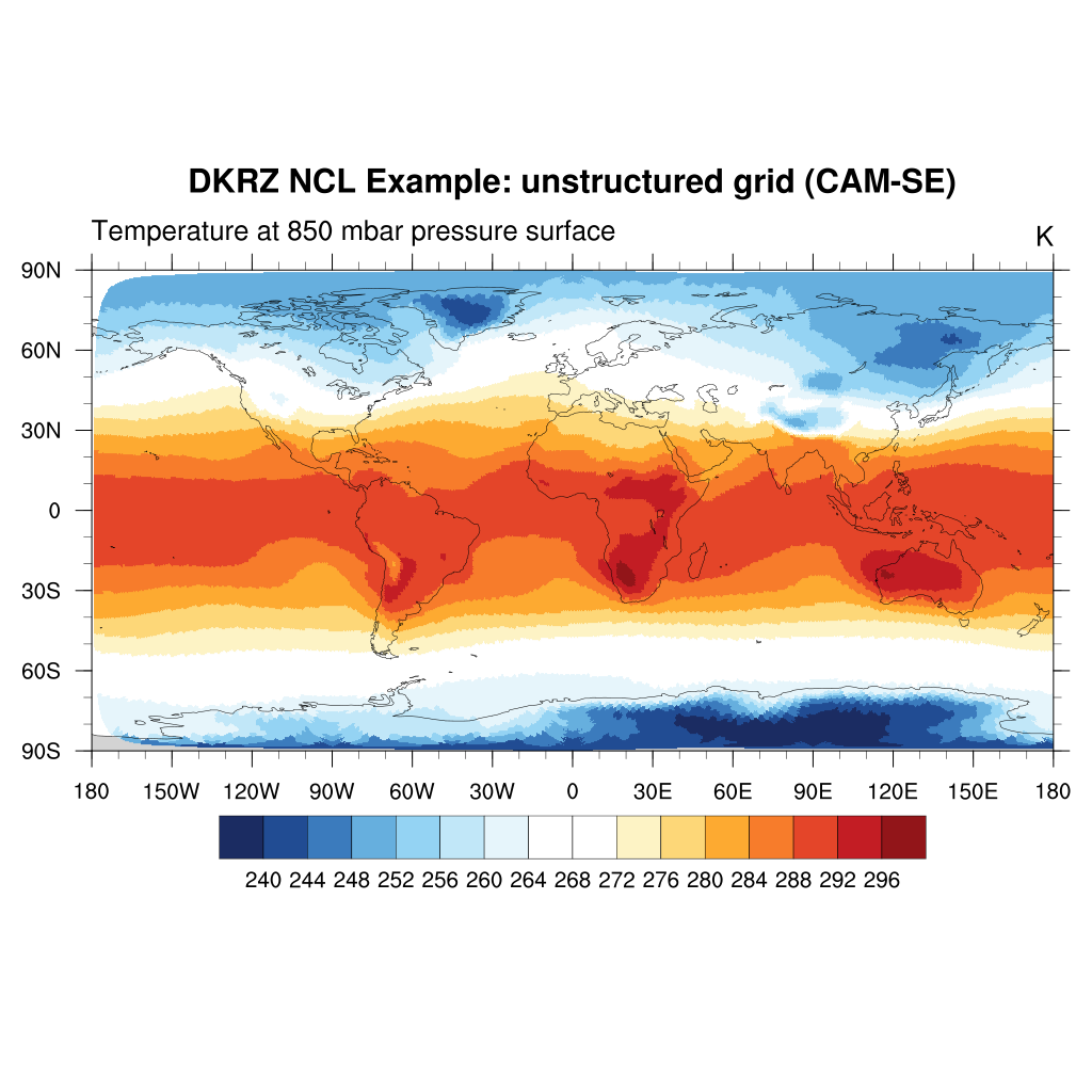
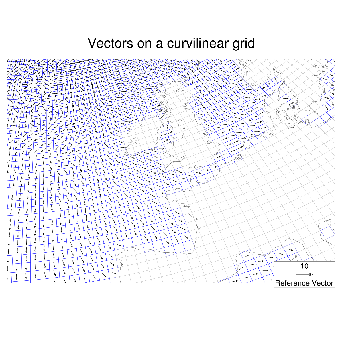
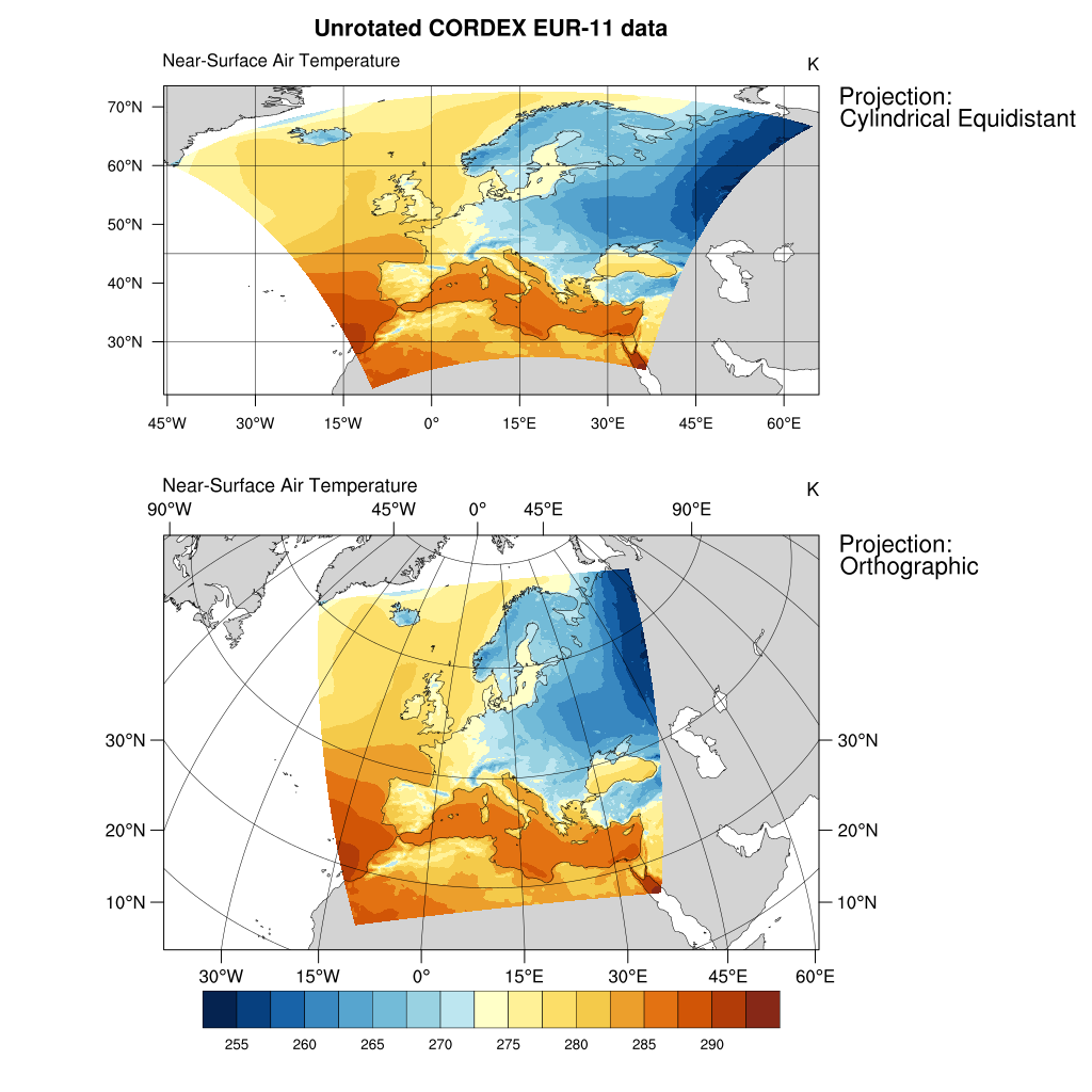
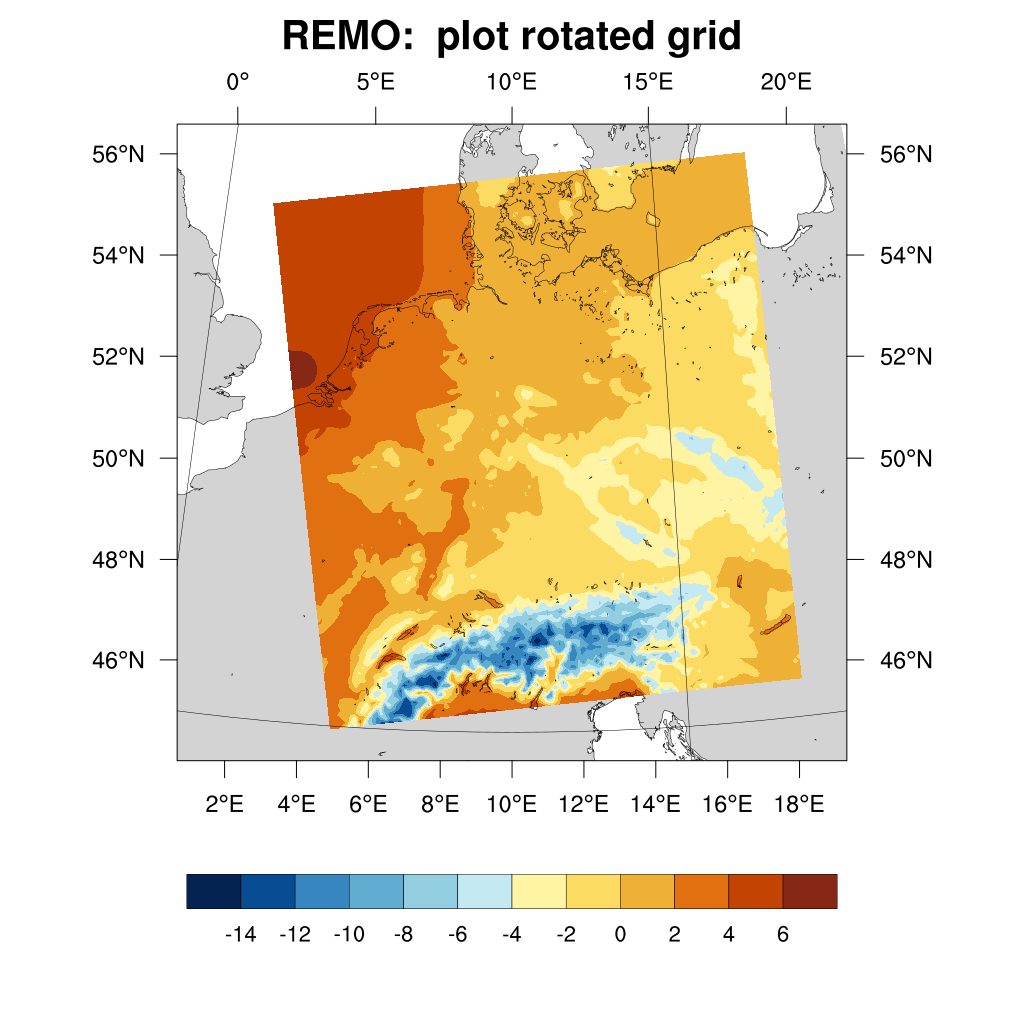
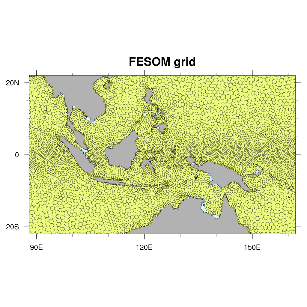
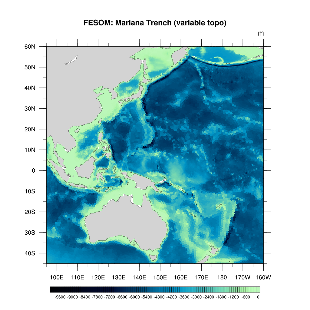
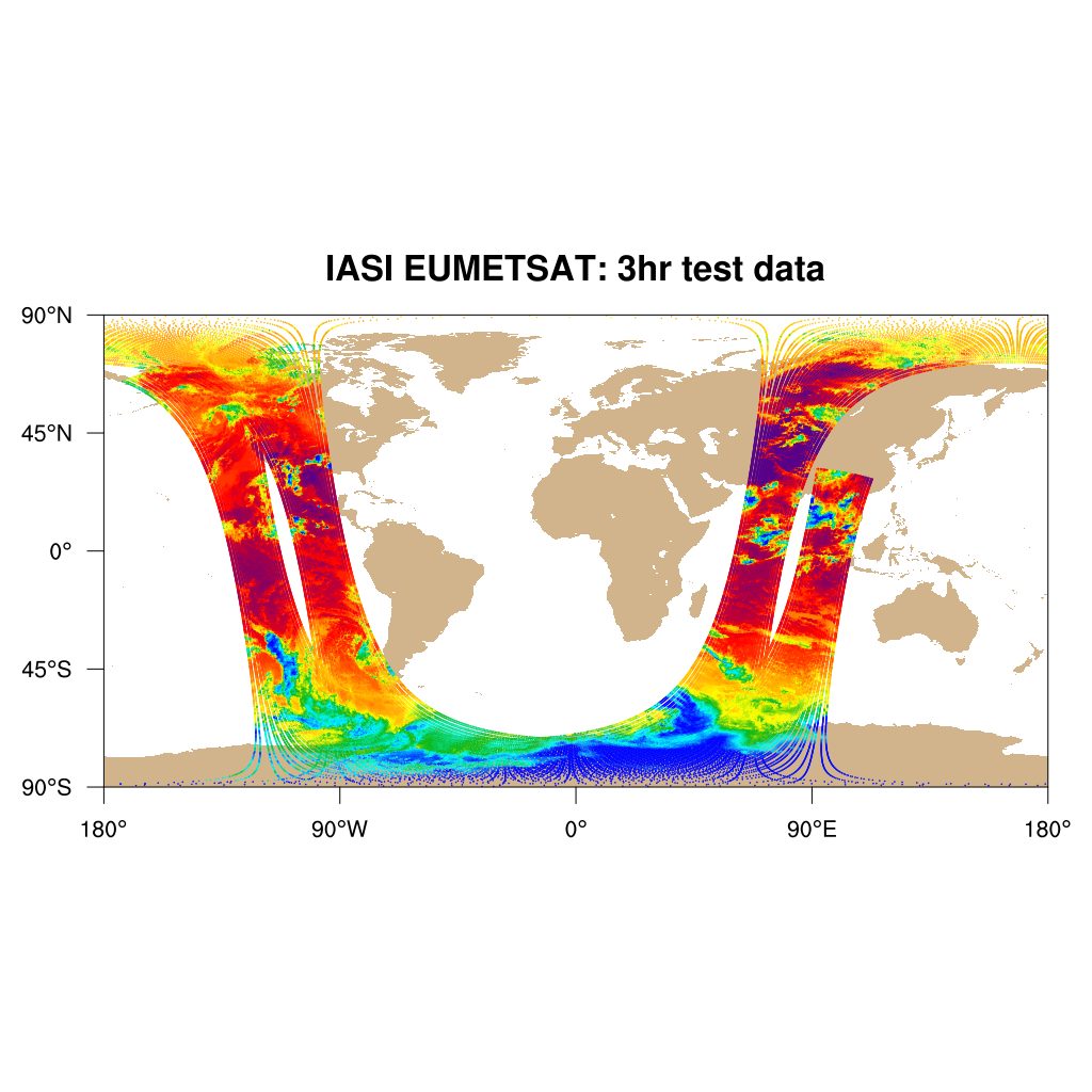
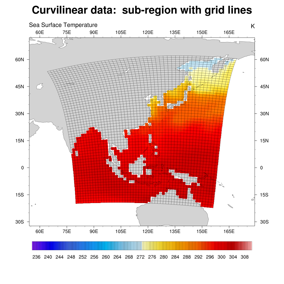
rectilinear, curvilinear, unstructured (ICON, satellite data) |
|
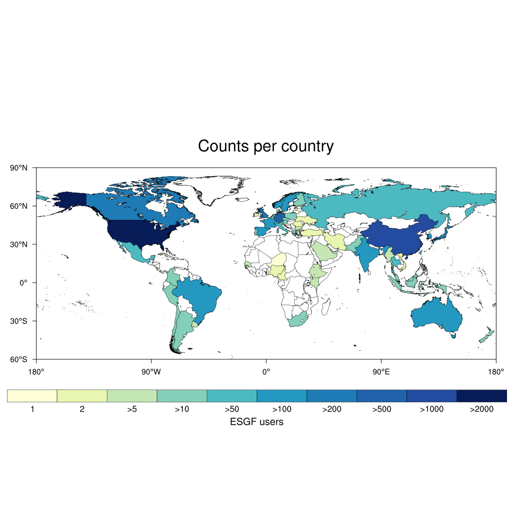
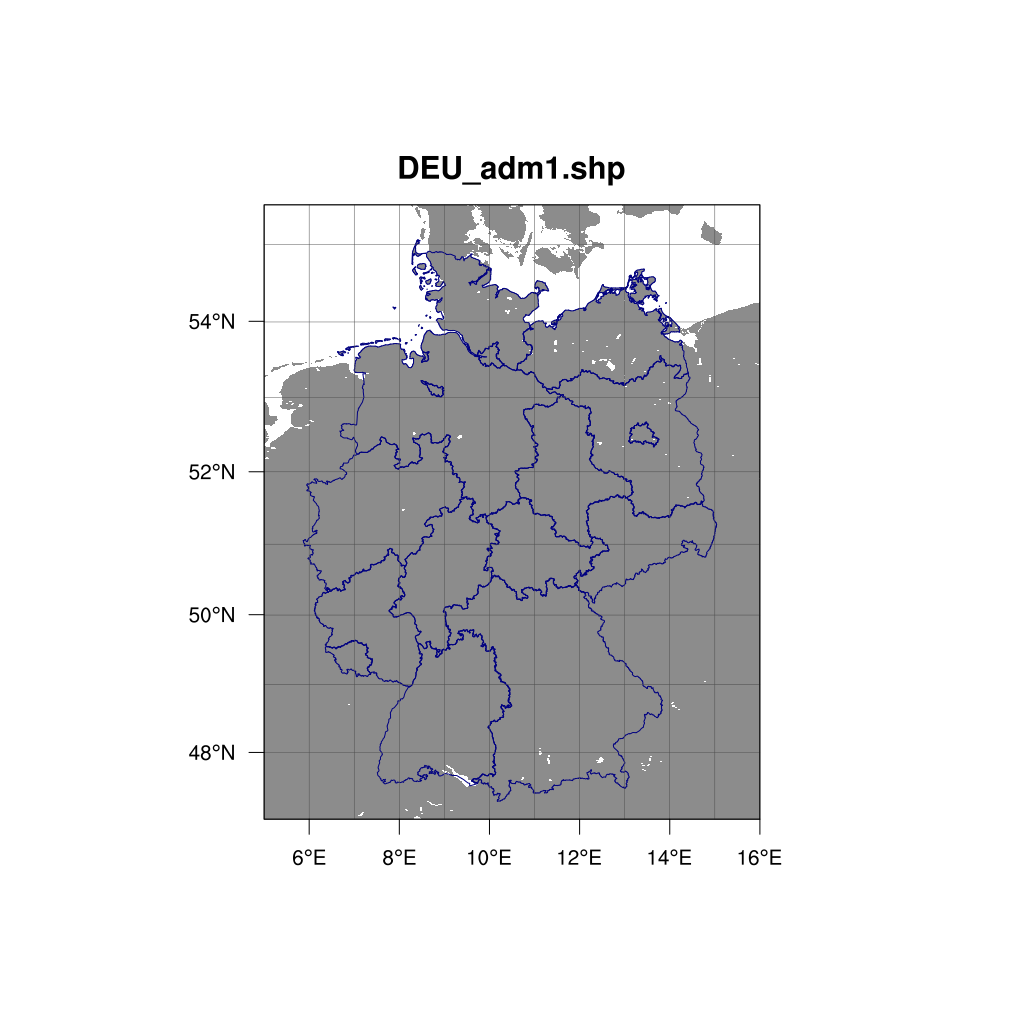
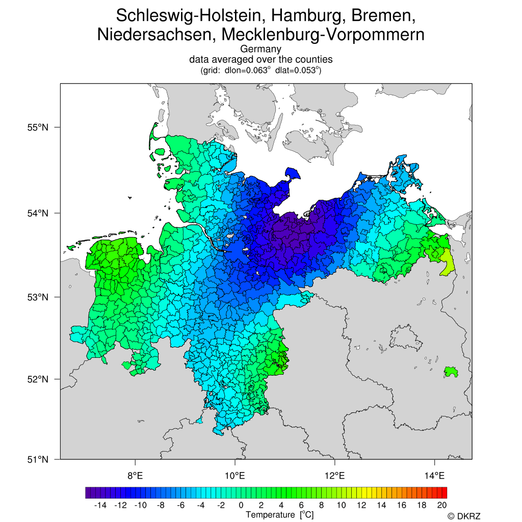
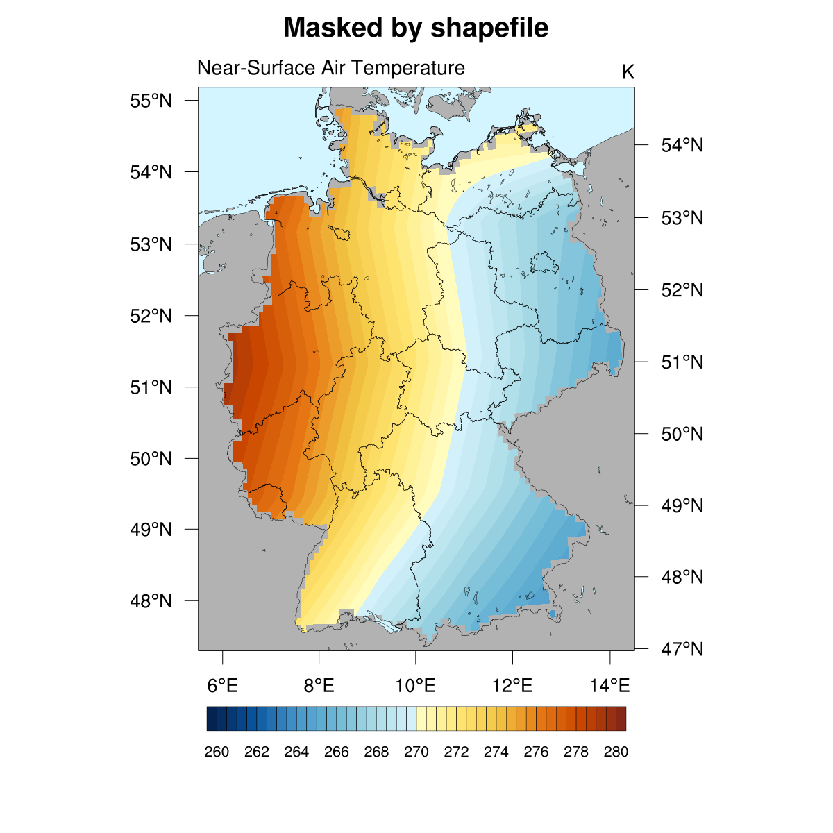
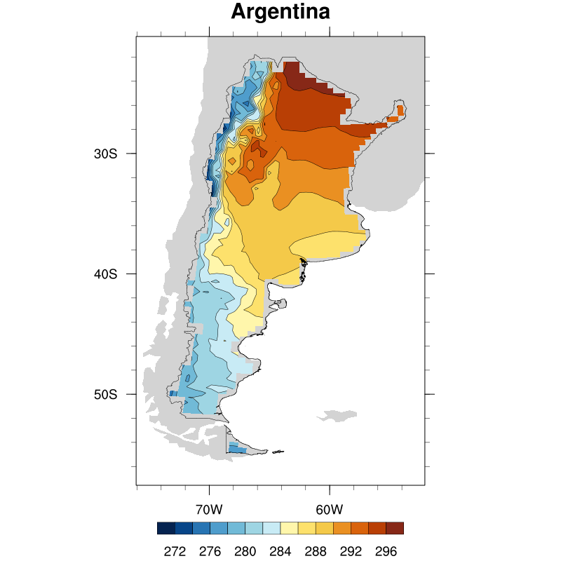
country outlines, compute temperature means of counties |
|
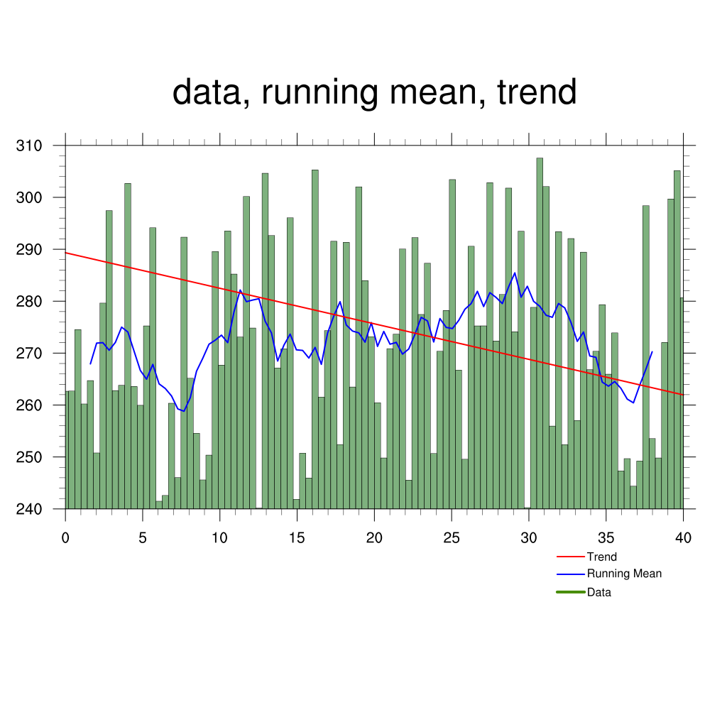
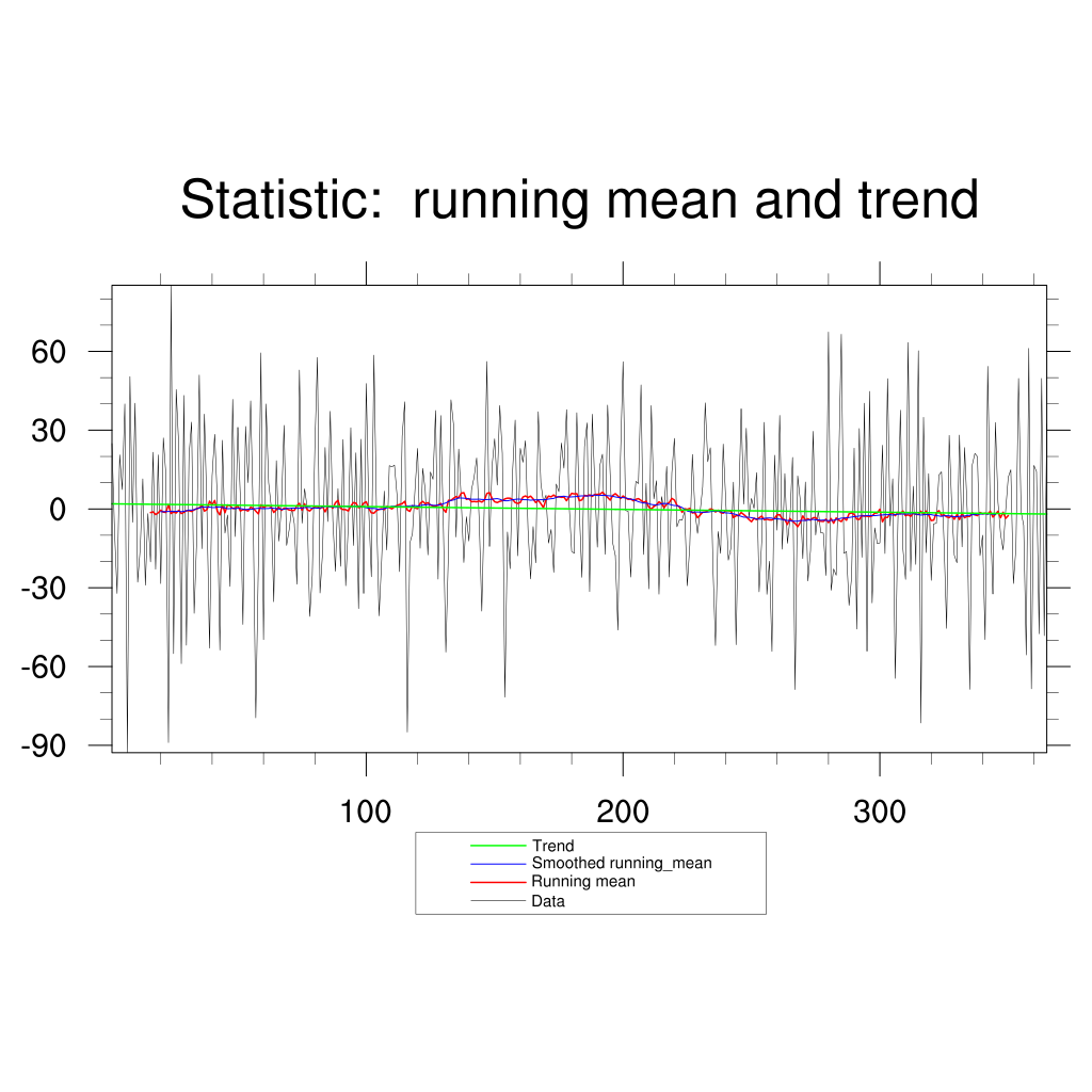
statistics: trend, running mean, averages, zonal mean |
|
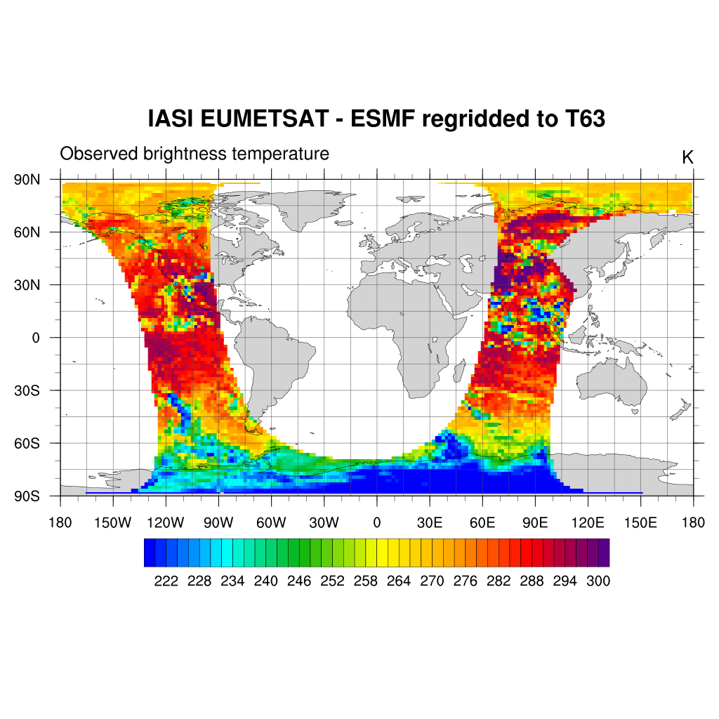
regrid curvilinear to rectilinear, regrid to higher resolution |
|
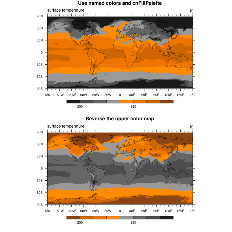
use of pre-defined color maps, named colors and opacity |
|
short and detailed version to write data to a new netCDF file |
|
how to use system function with double-quotes |
|
how to call/run an NCL script within a Shell script |
|
how use subprocess and subprocess_wait function |
|
miscellaneous scripts e.g. calendar conversion |
More examples can be found on the examples web page of NCL.
Maps#
XY-plots#

Contour plots#
Vector plots#
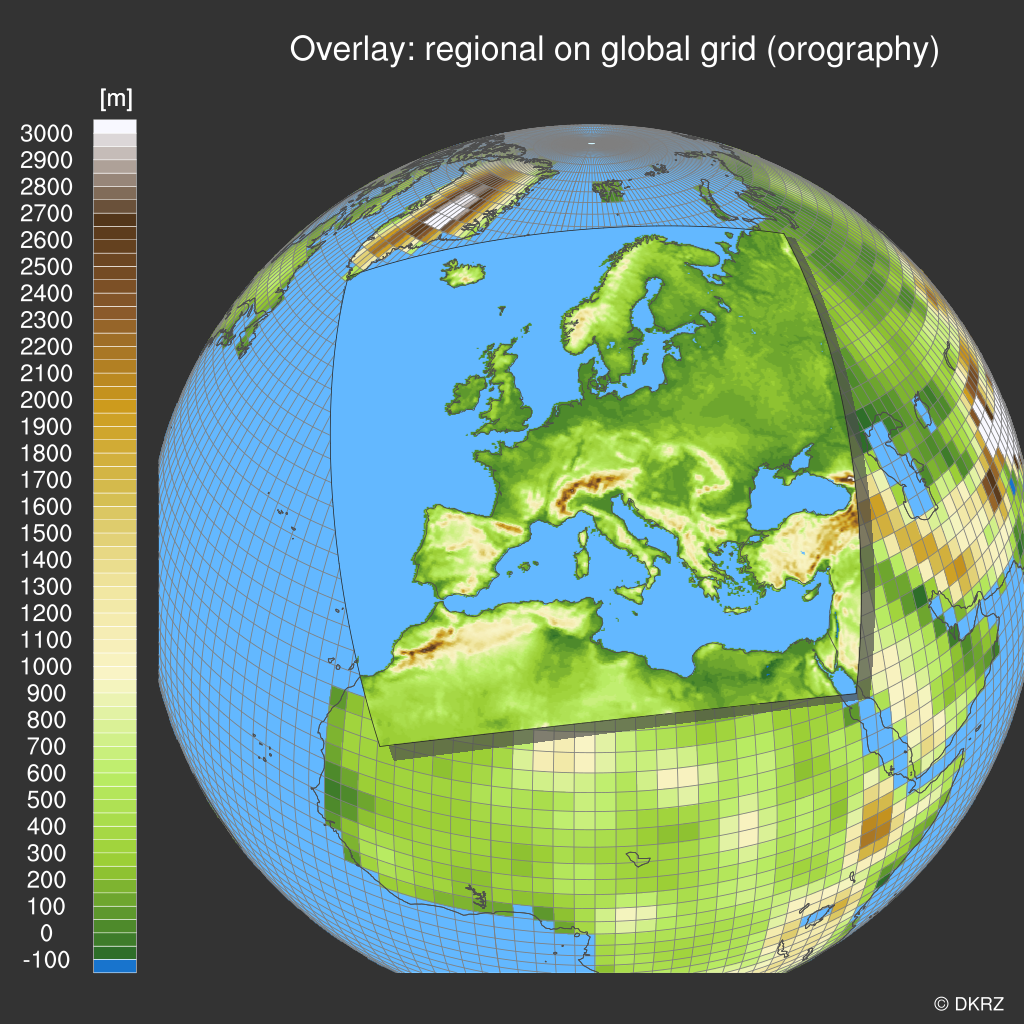
Overlays#
Annotations#

Panel plots#
Animations#
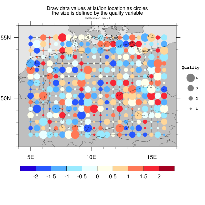
Special plots#
Grids#
Shapefiles#
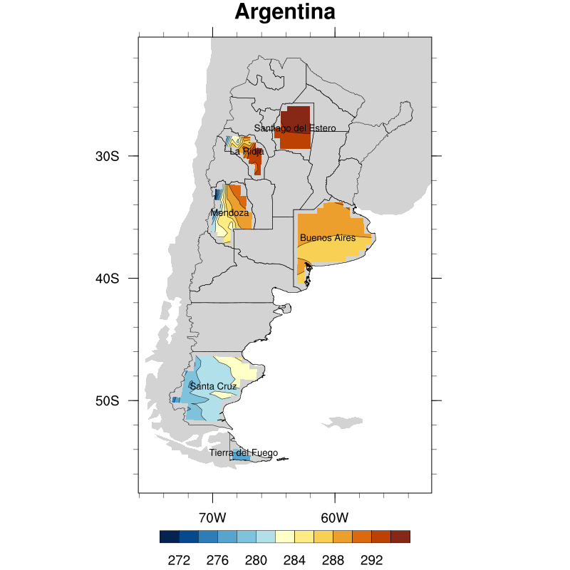
Analysis#
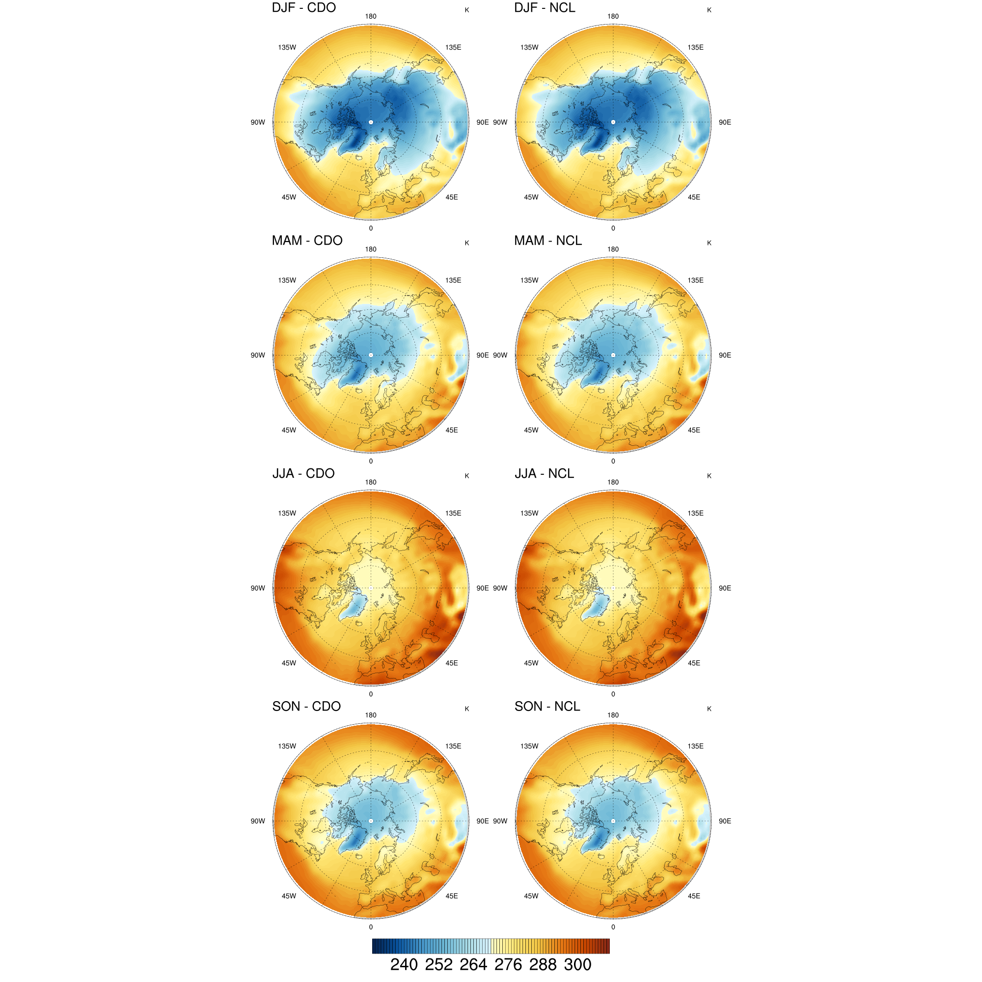
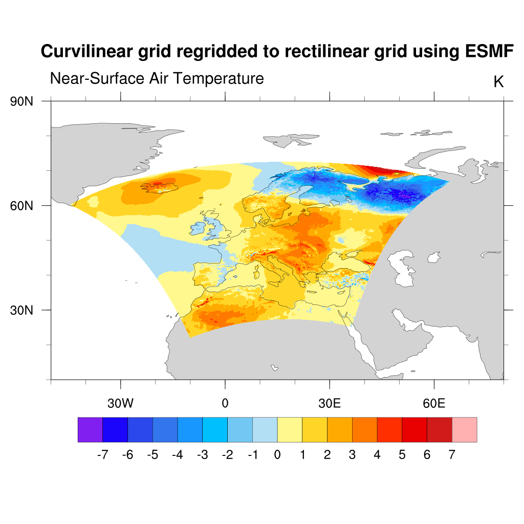
Regridding#
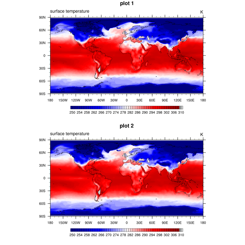
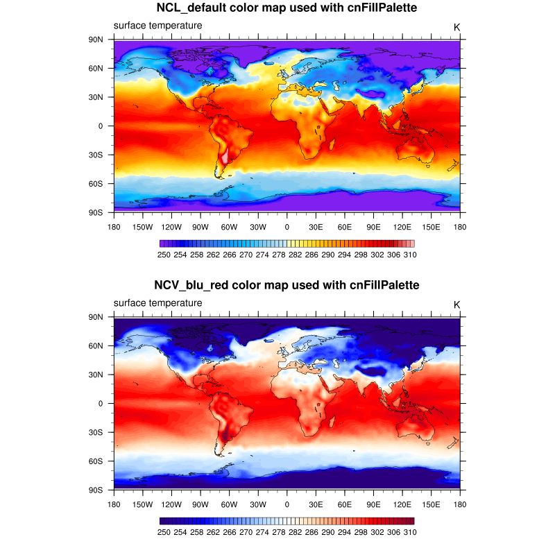
Colors#
Write netCDF file#
Export data to new netCDF file: short and simple
System calls#
system or systemfunc call with double quotes To execute a UNIX shell command within an NCL script the built-in system procedure or the systemfunc function can be used. system("date")
datestring = systemfunc("date")
To execute a shell command using double quotes itself you have to do a little trick to get the correct result. For example: system("date "+DATE: %Y-%m-%d%nTIME: %H:%M:%S"")
will cause an error like fatal:syntax error: function systemfunc expects 1 arguments, got 0
fatal:error at line 67 in file systemfunc_pass_variables.ncl
fatal:syntax error: line 71 in file systemfunc_pass_variables.ncl before or near :
system("date "+DATE:
-------------------^
fatal:error in statement
fatal:Syntax Error in block, block not executed
fatal:error at line 73 in file systemfunc_pass_variables.ncl
The trick is to define the double quote character as a variable with the built-in function str_get_dq() and use this variable with the concatenation operator + to create the command string for system or systemfunc: quote = str_get_dq()
datestring = systemfunc("date "+quote+"+DATE: %Y-%m-%d%nTIME: %H:%M:%S"+quote+" ")
print(datestring)
|
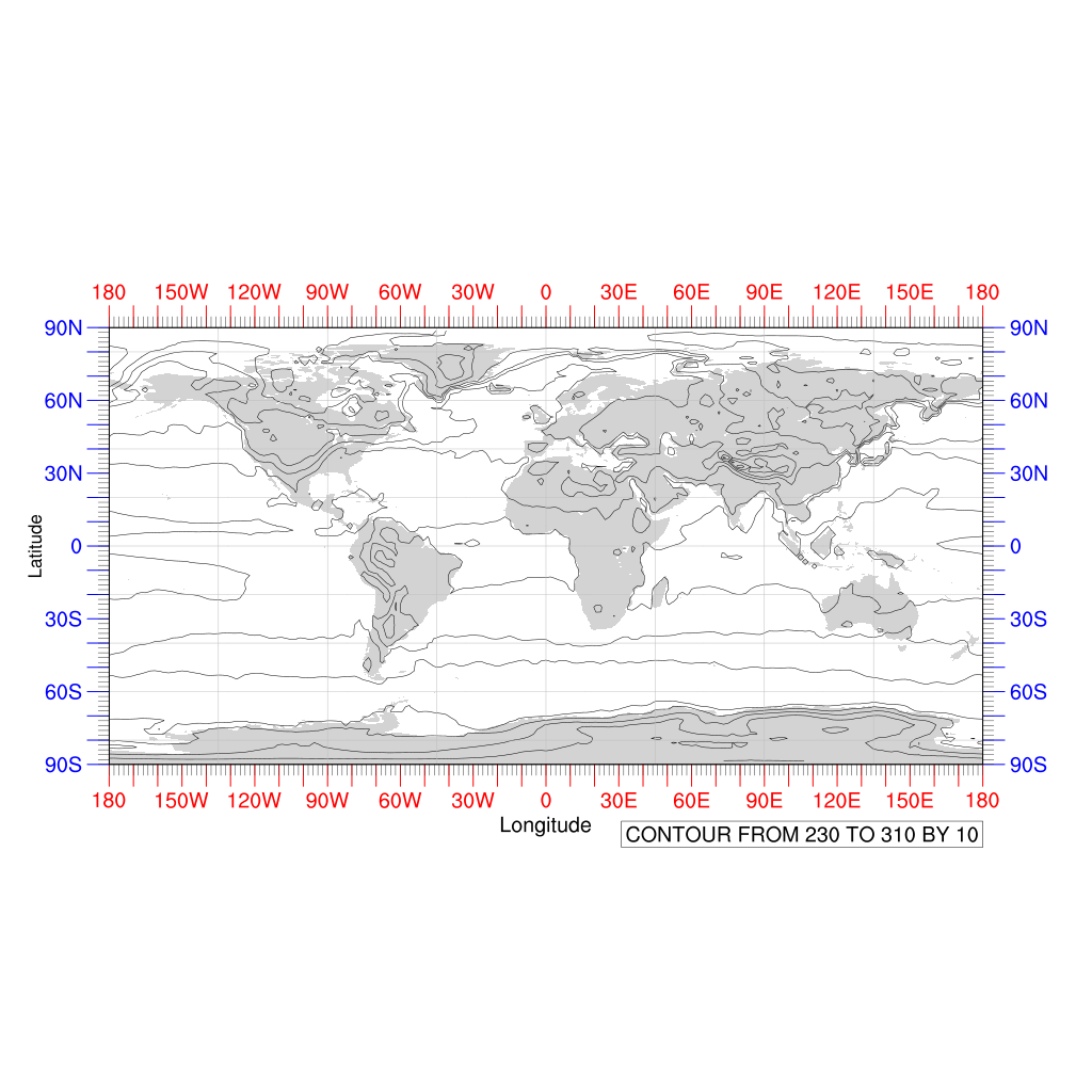
Command line parameter#
Run an NCL script from a shell script csh/tcsh snippet: ...
set cnfill = "True"
set country = "True"
set cmin = 255.0
set cmax = 300.0
set cint = 1
ncl -n -Q country=\""$country"\" \
cnfill=\""$cnfill"\" \
contours=\""${cmin},${cmax},${cint}"\" \
calls_from_batch_job_NCL_script.ncl
...
NCL script snippet: ...
if(isvar("cnfill")) then ;-- is 'cnfill' on command line?
mres@cnFillOn = True ;-- turn on color fill
mres@cnFillPalette = "rainbow"
mres@cnLineLabelsOn = False
mres@cnInfoLabelOn = False
mres@cnLinesOn = False
end if
if(isvar("country") .and. country .eq. "True") then ;-- is 'country' on command line?
mres@mpOutlineBoundarySets = "National" ;-- draw national outlines
end if
if(isvar("contours")) then ;-- is 'contours' on command line?
cmin = tofloat(str_get_field(contours,1,","))
cmax = tofloat(str_get_field(contours,2,","))
cint = tofloat(str_get_field(contours,3,","))
mres@cnLevelSelectionMode = "ManualLevels" ;-- contour min, max and interval
mres@cnMinLevelValF = cmin
mres@cnMaxLevelValF = cmax
mres@cnLevelSpacingF = cint
else ;-- set defaults
cmin = min(data)
cmax = max(data)
clevs = 18
mnmxint = nice_mnmxintvl( cmin, cmax, clevs, False)
mres@cnLevelSelectionMode = "ManualLevels"
mres@cnMinLevelValF = mnmxint(0)
mres@cnMaxLevelValF = mnmxint(1)
mres@cnLevelSpacingF = mnmxint(2)
end if
...
|
Task parallelism#
Use an NCL script to start running multiple NCL plot scripts at one time in parallel.
The main script running multiple plot scripts using the subprocess function and wait until their are finished using subprocess_wait.
;---------------------------------------------------------------
;  main_subprocess.ncl
;
;  Use the subprocess and subprocess_wait functions to generate
;  the time dependend PNG plots to create an animation.
;
;  This script is calling the plot script
;                 plot_script.ncl
;
;  Use the max_processes variable to set the number of processes
;  running in parallel. A number equal to the number of processor
;  cores can be a good choice.
;---------------------------------------------------------------
begin
  st = get_cpu_time()

;-- create a directory for the plots, if it doesn't exit
  system("mkdir -p test_subprocess_images")

;-- initialize number of timesteps and set maximum number of processes
;  ntsteps       = -1
  max_processes = 8

;-- open the file and retrieve the number of timesteps
  f    = addfile("rectilinear_grid_2D.nc", "r")
  time = f->time

  ntsteps = dimsizes(time)
  print("timesteps: "+ntsteps)

  ndone   = 0
  nactive = 0

;-- only max_processes at a time
  do i=0,ntsteps-1
     do while (nactive .ge. max_processes)
        pid = subprocess_wait(0,True)   ;-- check for completition
        if (pid .gt. 0) then
           ndone   = ndone + 1
           nactive = nactive - 1
           break
        end if
     end do

     print("plot: "+i)

     cmd = "ncl plot_script.ncl " + str_get_sq() + "tstep=" + i + str_get_sq() + " >/dev/null"

     pid = subprocess(cmd)

     nactive = nactive+1
  end do

;-- check if we have to wait until all jobs are done
  do while (ndone.lt.ntsteps-1)
     pid = subprocess_wait(0,True)      ;-- check for completition
     if (pid.gt.0) then
        ndone = ndone + 1
     end if
  end do

;-- how long does it take
  et = get_cpu_time()
  print("--> Plots CPU time:  "+ (et-st) + " seconds")

;-- create the animated GIF file
  system("cd test_subprocess_images; convert -delay 100 -loop 0 plot_tsurf*.png animation.gif")

;-- that's it
  et = get_cpu_time()
  print("--> GIF CPU time:    "+ (et-st) + " seconds")

end
Plot script called by the main script:
;---------------------------------------------------------------
;  plot_script.ncl
;
;  Create a contour plot of variable tsurf at a given time and
;  save it to the directory test_subprocess_images. For each time
;  step the variable tstep has to be given on the command line.
;---------------------------------------------------------------
begin
  f     = addfile("rectilinear_grid_2D.nc","r")
  var   = f->tsurf(tstep,:,:)

  date  = cd_calendar(f->time(tstep),0)
  title = sprinti("%04d",toint(date(0,1)))+"/"+sprinti("%4d",toint(date(0,0)))

  pltname = "test_subprocess_images/plot_tsurf"+sprinti("%04d",tstep)

  wks = gsn_open_wks("png",pltname)

  res                          =  True
  res@gsnMaximize              =  True

  res@tiMainString             =  title

  res@cnFillOn                 =  True

  res@lbOrientation            = "Vertical"
  res@pmLabelBarOrthogonalPosF =  -0.02

  plot = gsn_csm_contour_map(wks,var,res)

end
Miscellaneous#
Several helpful scripts e.g. to convert data using Julian calendar to a standard calendar.
a) Convert data using Julian calendar to standard calendar –> script