Extrusion of topography and bathymetry#
Using ParaView’s Calculator filter, surfaces can easily be extruded, as the following examples for Equidistant Cylindrical and Spherical Projection illustrate.
Equidistant cylindrical representation#
iHat * coordsX + jHat * coordsY + (z_ifc/9000.0 * ( kHat * (1+coordsZ)))Steps:
File -> Open… -> surface_1.nc
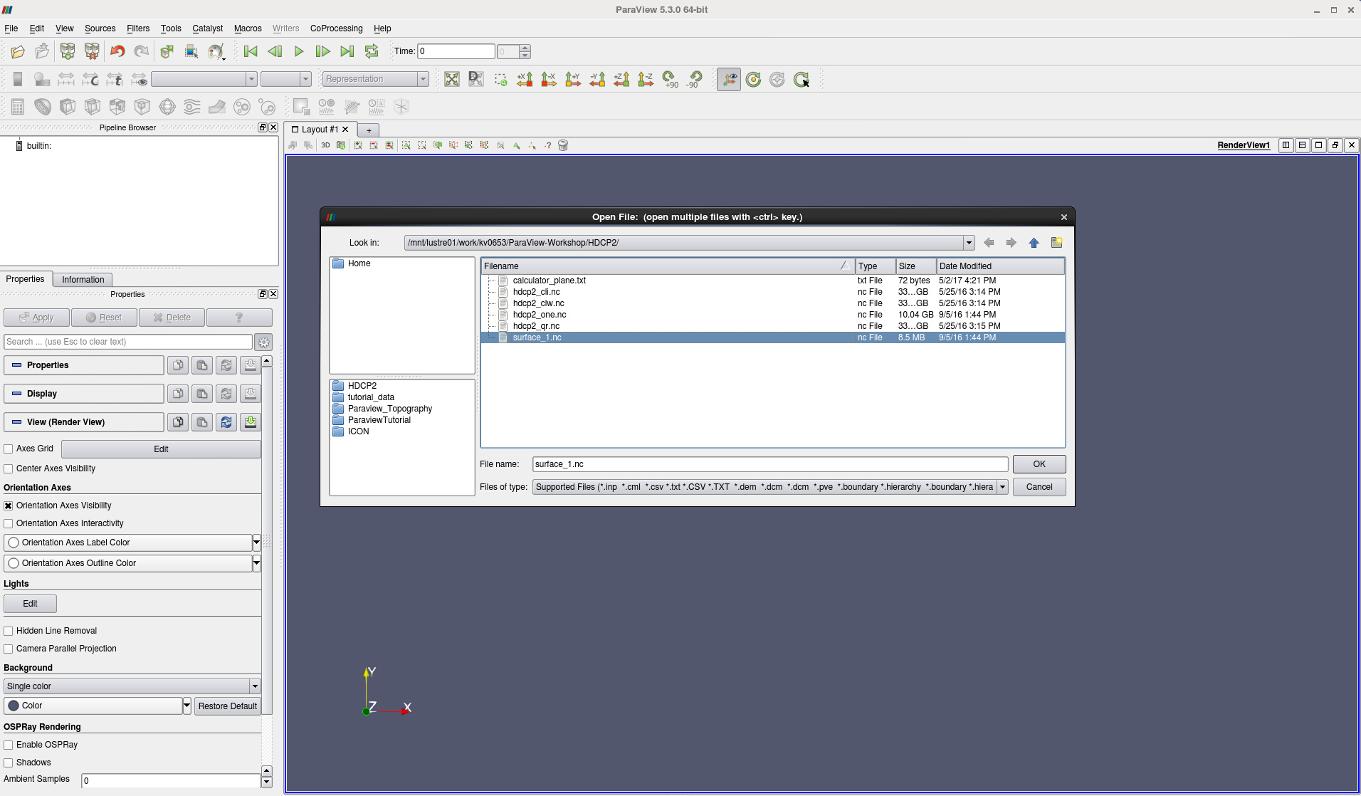
Figure 1: Open data surface_1.nc .
Select NetCDF files generic and CF conventions
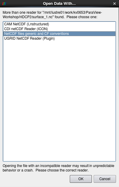
Figure 2: Select reader NetCDF files generic and CF conventions .
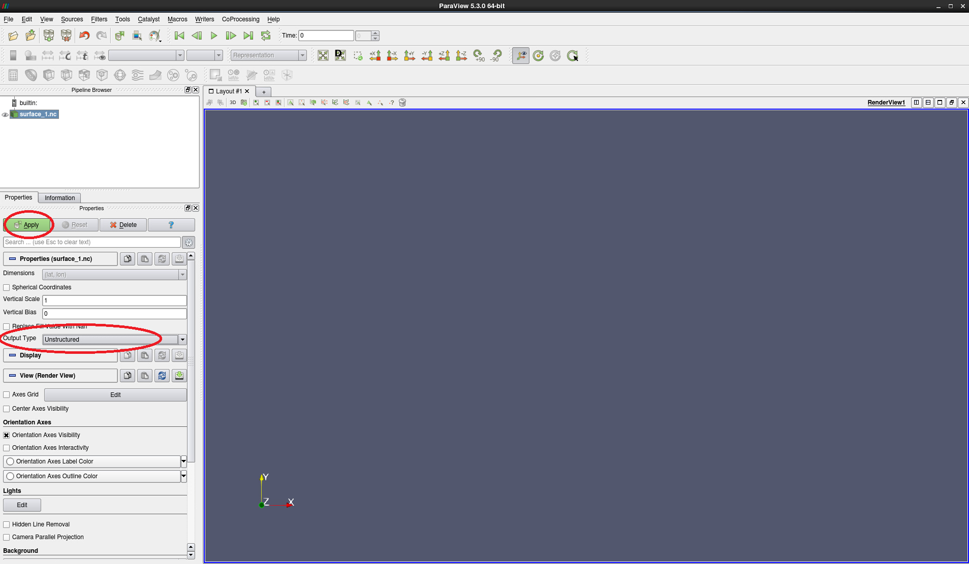
Figure 3: Select Output Type Unstructured .
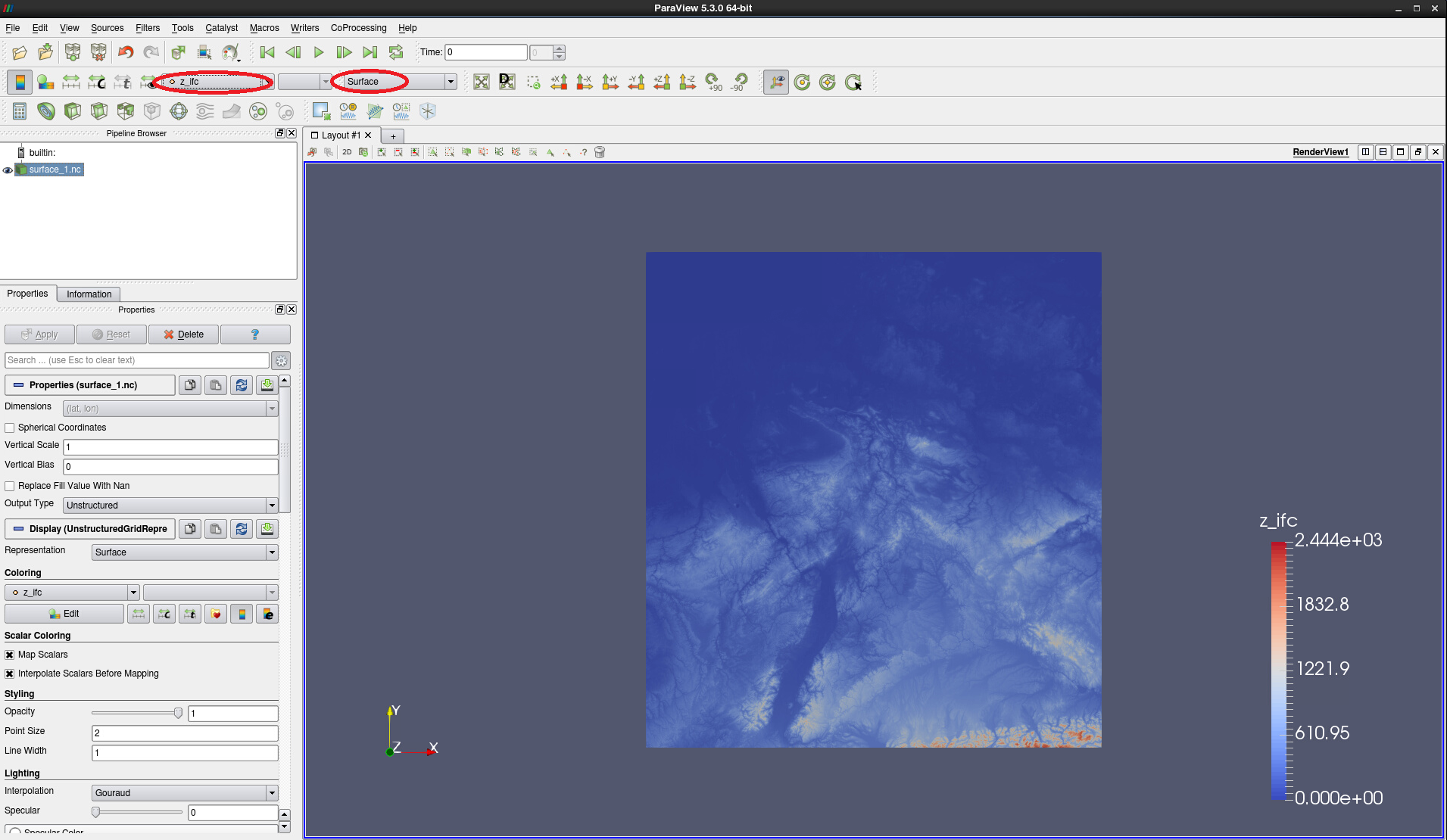
Figure 4: z_ifc displayed as Surface
Select Calculator filter by clicking on the Calculator symbol in the toolbar and choose the following settings:
Attribute Mode: Point Data
X Coordinate results
Enter extrusion formula
X Replace invalid results
Click Apply
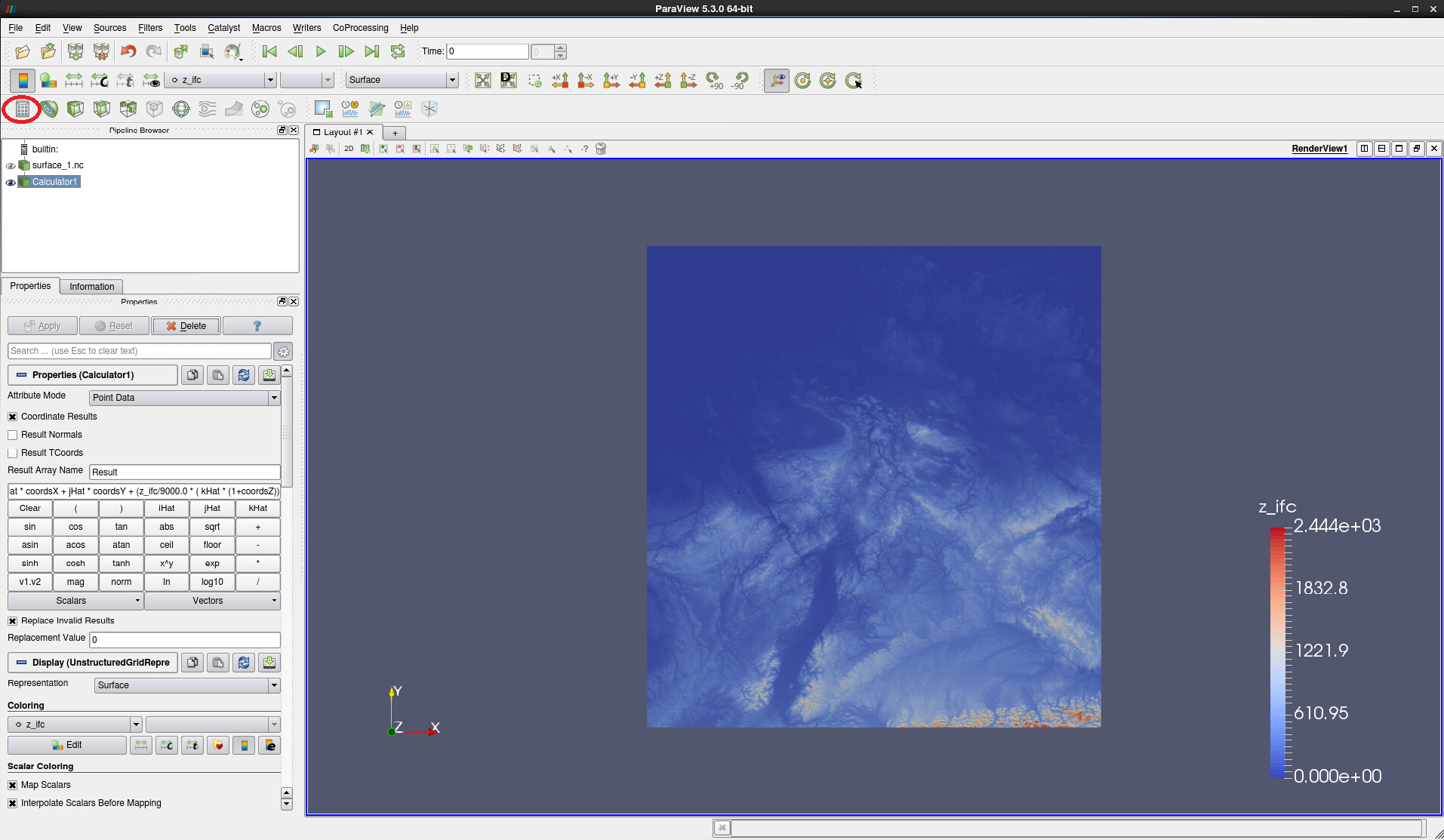
Figure 5: Calculator filter after surface height extrusion
To change the coloring of the extruded data, select the Calculator module in the Pipeline and scroll down to the coloring section of the Calculator Properties. Use the button Choose preset (folder with a heart - see Fig. 6) to get to the overview of color presets shown in Fig. 7.
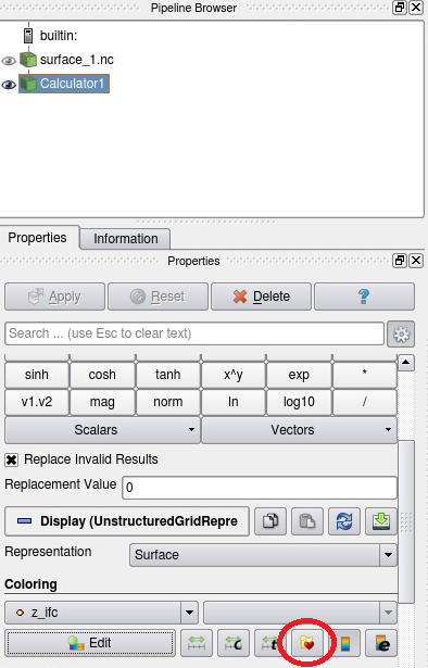
Figure 6: Choose colormap preset
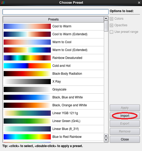
Figure 7: Import colormap preset
Press Import, navigate to a colormap .json file of your choice (e.g. color_surface.json - see Fig. 8 ) and press OK.
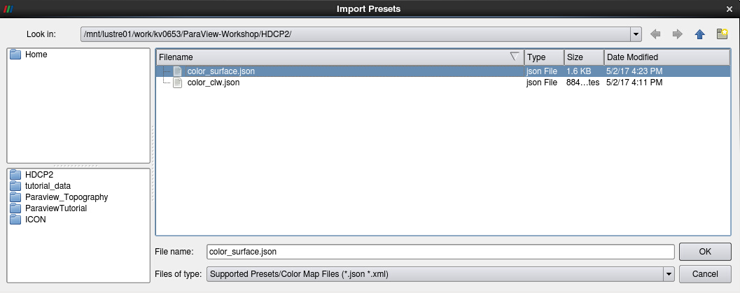
Figure 8: Import presetcolor_surface.json
Back in the Choose preset menu, the imported preset (here:Preset 3) is already selected and will be used upon clicking theApply button.When applied, press Close.
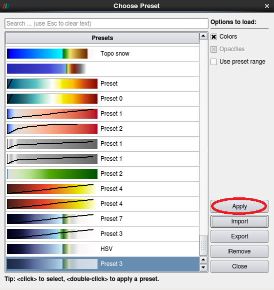
Figure 9: ClickApply with new preset selected
This yields the land surface representation shown in in Fig. 10.
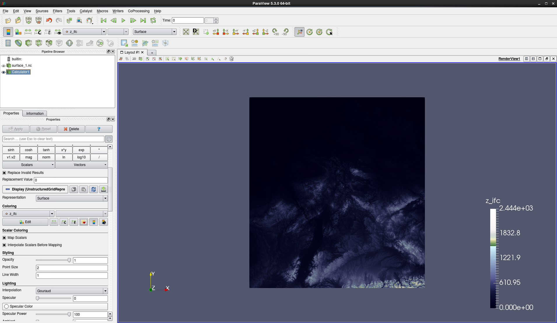
Figure 10: Colormap :file:`color_surface.json` applied to extruded topography
ParaView has automatically selected the minimum and maximum values of z_ifc as colormap limits. As the colormap is designed for the topography and bathymetry of the entire earth, it is necessary to adjust the colormap range accordingly.
To set an upper and lower colormap limit, click on the button Rescale to custom range (time bar with a black c - see Fig. 11) in the Coloring section of the Calculator Properties.
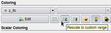
Figure 11: Button rescale to custom range
In the Set range window, enter -10000 as minimum and 6306 as maximum values (see Fig. 12) and hit rescale.
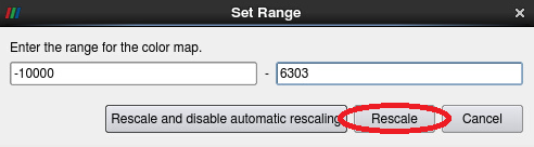
Figure 12: Window for setting the custom range
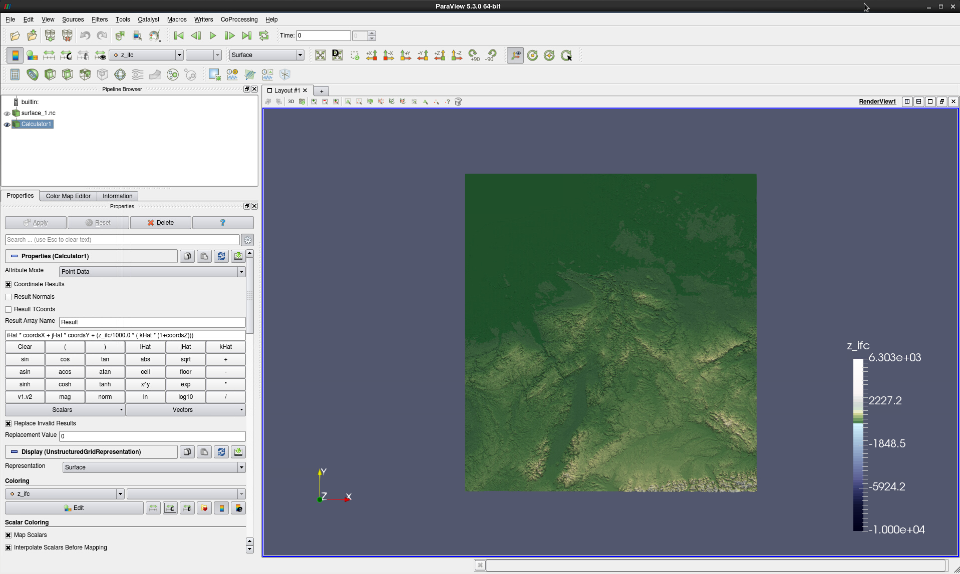
Figure 13: Data colored by :file:`color_surface.json` and custom range -10000 to 6303
To achieve the result shown in Fig. 14, with the ocean colored in light blue and land colored in shades of green, you need to edit the Color transfer function values in the Colormap Editor. For convenience and for HD(CP)² data over Germany we suggest that you load the existing state file land_surface.pvsm prior to loading your data of interest.
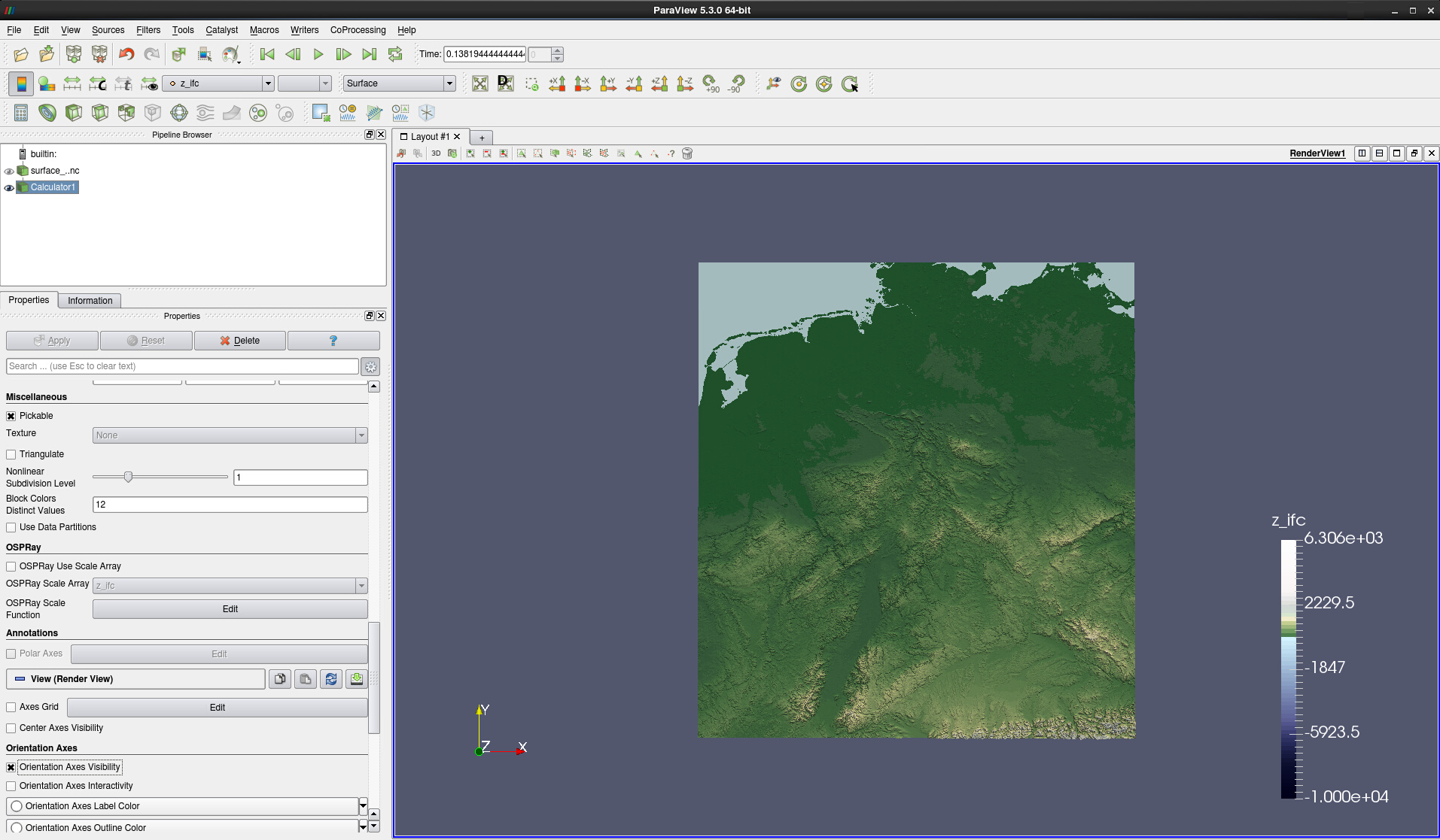
Figure 14: Land surface height with realistic ocean and land coloring
Last but not least: If you would like to change the colormap labeling, press the button Edit colormap legend properties (colormap symbol and black e - see Fig. 6) in the Coloring section of the Calculator Properties.
Spherical representation#
ETOPO data provided by NOAA is a suitable for extruding global topography and bathymetry data in a spherical projection. In this example we are going to use an ETOPO texture in the VTK Polydata format (.vtp). However, we might just as well use a netCDF data file.
(1 + (altitude/6370000) * 100)* ( iHat * cos(asin(coordsZ)) * cos(atan(coordsY/coordsX)) * coordsX/abs(coordsX) + jHat * cos(asin(coordsZ)) * sin(atan(coordsY/coordsX)) * coordsX/abs(coordsX) + kHat * coordsZ )Steps:
File -> Open…
Navigate to
topography.vtp, click OK.Press Apply in the Properties of topography.vtp
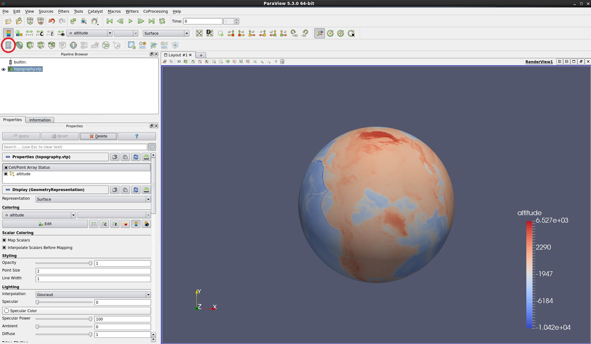
Figure 15: Altitude displayed as Surface
Select Calculator filter by clicking on the Calculator symbol in the toolbar and choose the following settings:
Attribute Mode: Point Data
X Coordinate results
Enter extrusion formula
X Replace invalid results
Click Apply
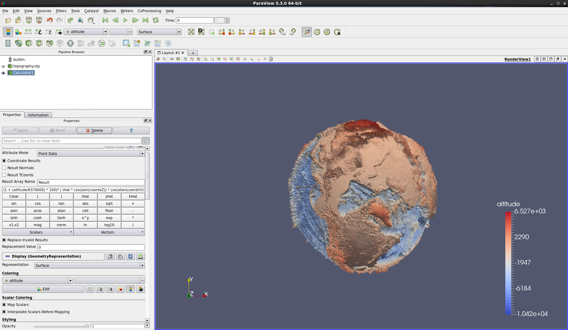
Figure 16: Altitude extruded
Load the colormap topography_color.json via Choose Preset and Import (see above for details). The result is shown in Fig. 17.
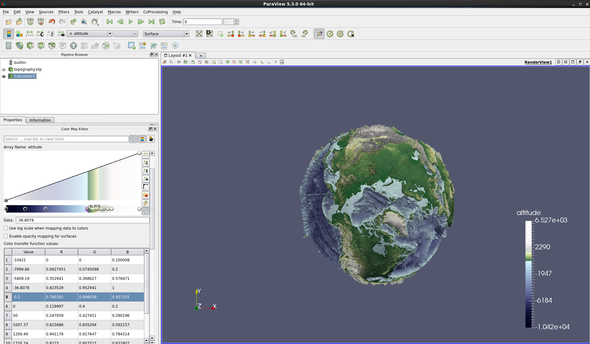
Figure 17: Colormap topography_color.json applied
In the Colormap Editor, you can click on one of the control points in the Color transfer function editor to show the table of Color transfer function values. Here you can see which data values have RGB values defined. Double-click on a control point to see its color or look up the respective RGB values in an RGB Color Code Charts. For the current colormap and dataset, data value of -0.2 m is shaded in blue while a value 0 m has a green color assigned.
Save your project as a ParaView state file in a directory where you have write access, e.g. as spherical_earth_orography.pvsm.
Coastlines for spherical representation#
/work/kv0653/ParaviewTutorial/coastlines.vtkWorld_Coastlines_and_Lakes.vtpSteps:
1. File -> Open… coastlines.vtk (see Fig. 18)
- Click OK
- Click Apply
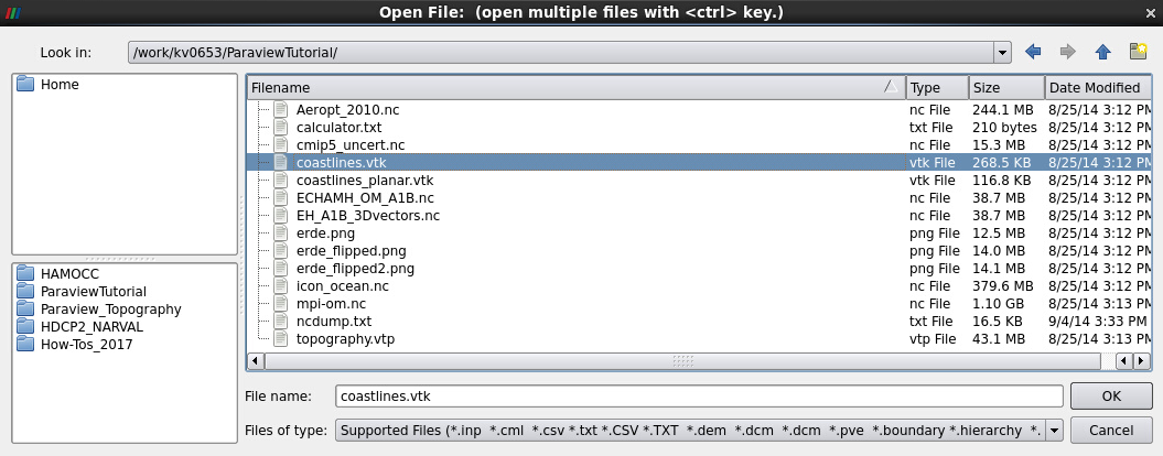
Figure 18: Open coastlines.vtk
For an equidistant cylindrical projection of the earth, you would use the file coastlines_planar.vtk instead. To find out more about this, have a look at the ParaView tutorial document. Fig. 19 shows the result of applying coastlines.vtk. The coastlines are very thin and do not exactly match the transition from land to water as indicated by the colormap. Moreover, the coastlines are quite coarse and angular, as looking at the coastlines only (see Fig. 20) shows.
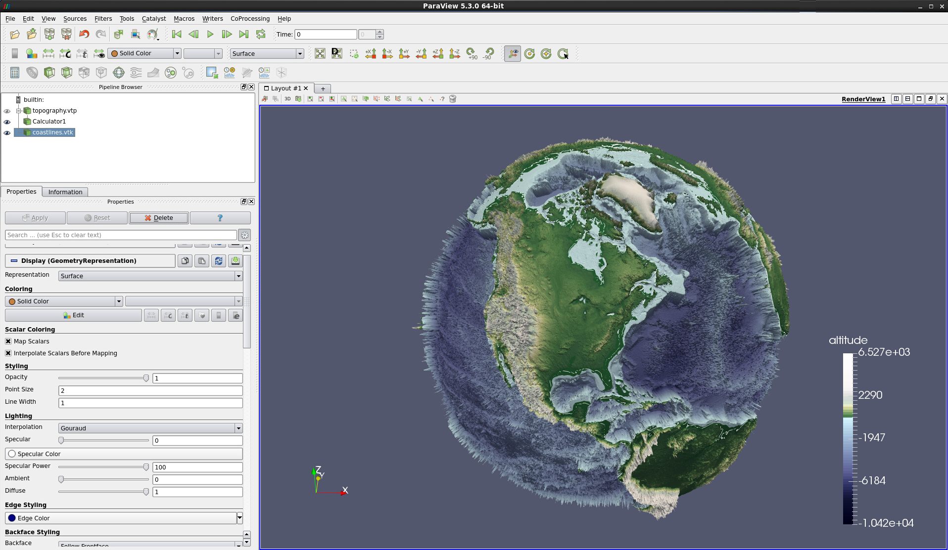
Figure 19: coastlines.vtk applied
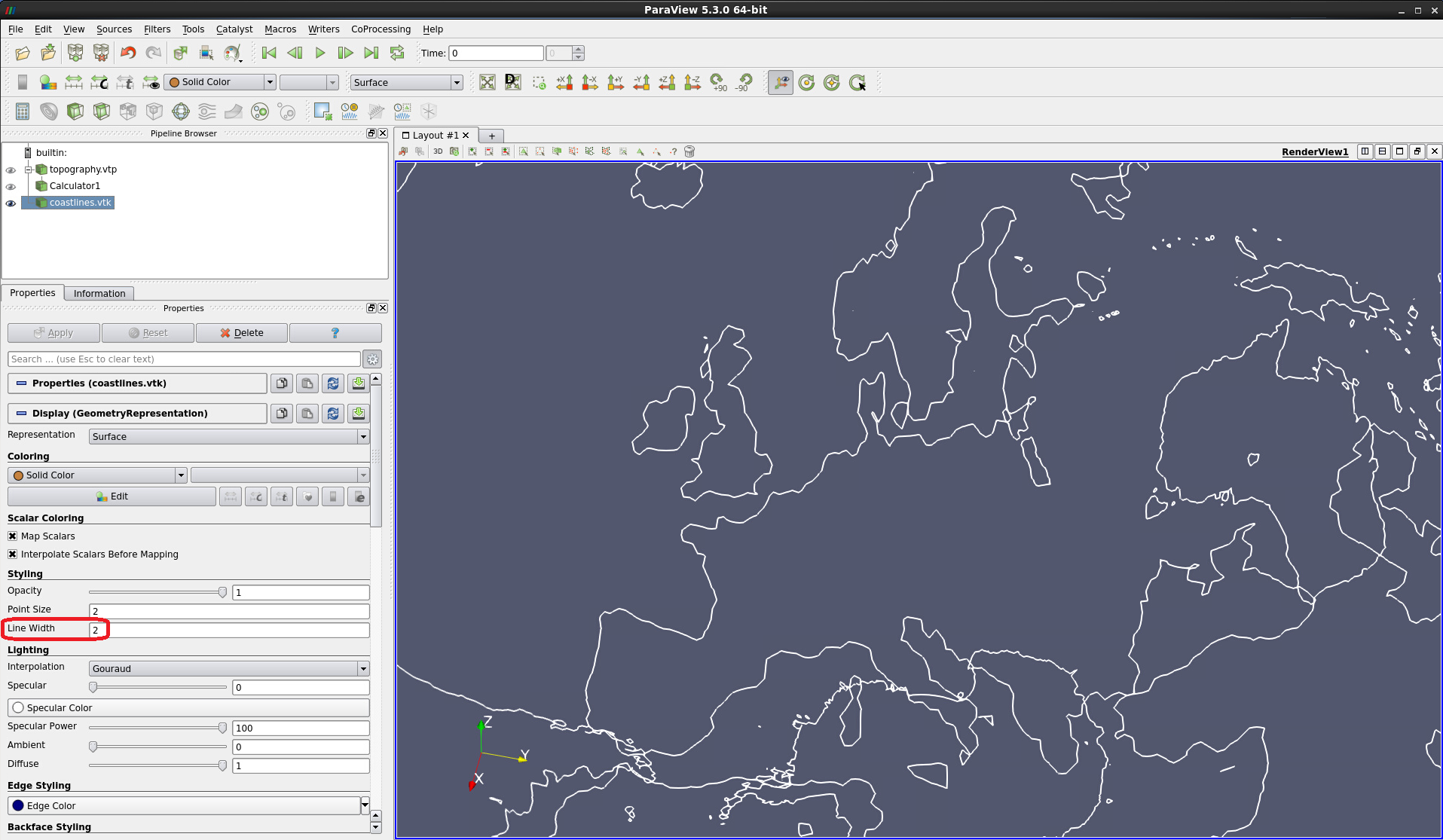
Figure 20: Displaying only the coastlines with line width increased to 2.
To have the coastlines displayed on top of the topography (see Fig. 21):
2. In the coastlines.vtk module, scroll down to the Transforming section and enter 0.002 in the third field behind
Translation (see Fig. 21).
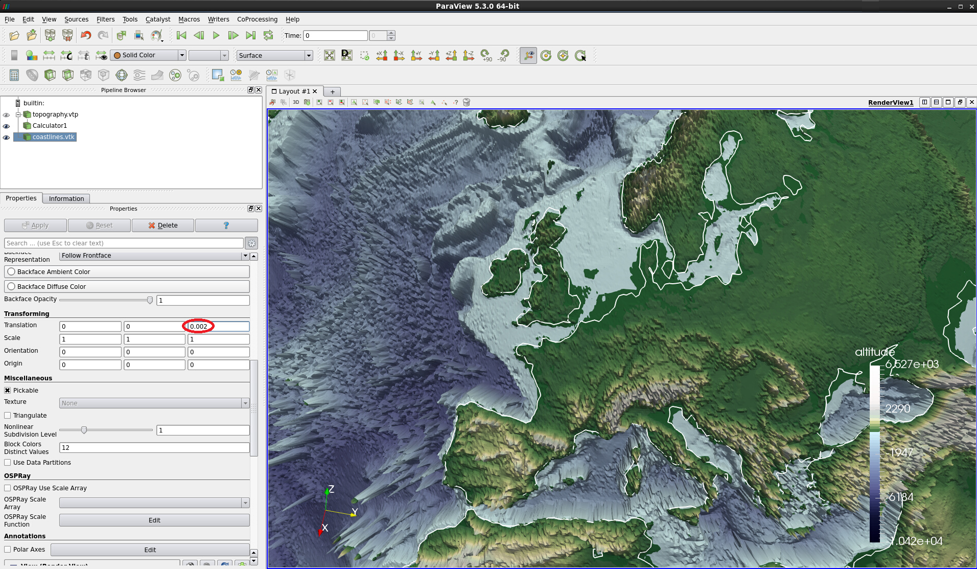
Figure 21: Coastlines translated vertically by 0.002
To further improve the appearance of the coastlines we suggest that you use the coastline data set World_coastlines_and_Lakes.vtp instead (see Fig. 22) and adjust the colormap for the Calculator1 module to achieve a better match between coastlines and the transition between ocean and land colors (not shown here).
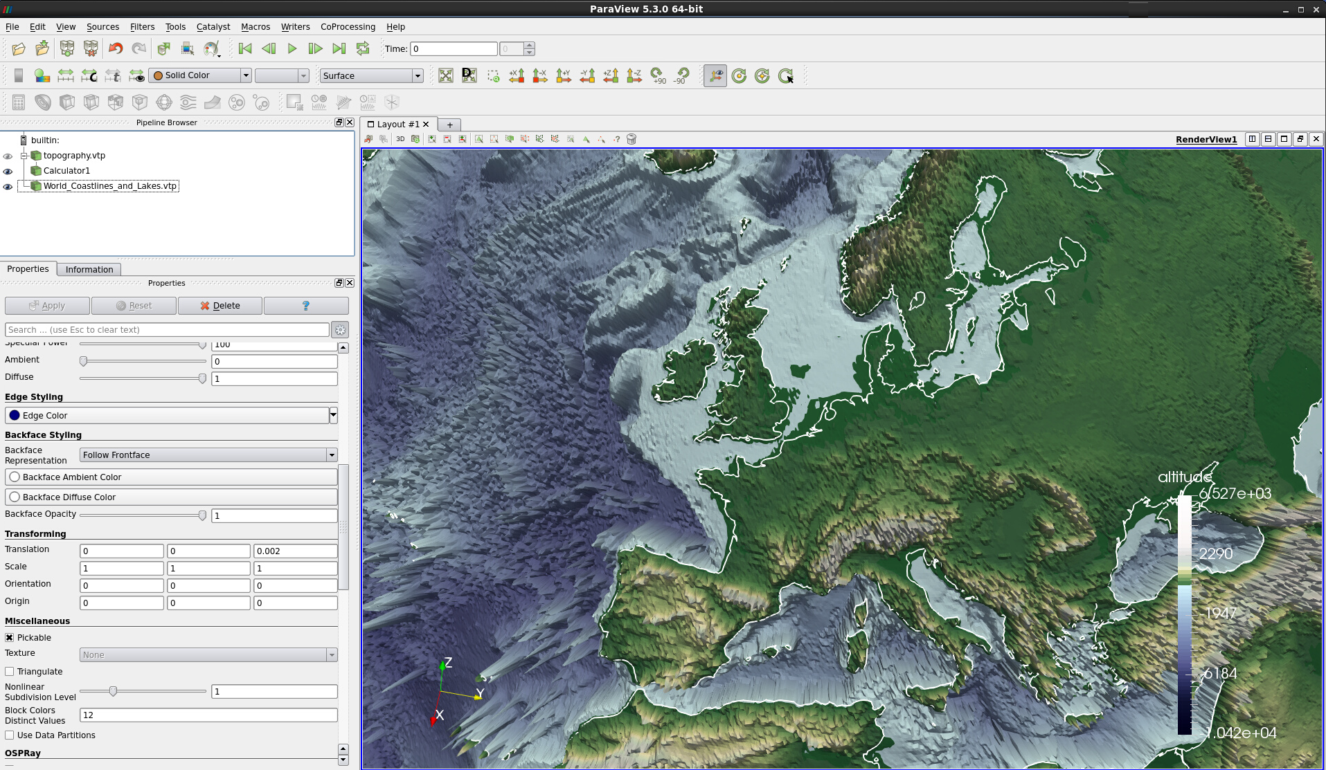
Figure 22: Higher resolution coastlines translated vertically by 0.002
When done, remember to save your project as a state file.
If you are interested in mapping an earth texture to the extruded surface of the earth, scroll down to the bottom part of this tutorial.